Fluid Mechanics · Hazen-Williams Equation
Hazen-Williams Equation Formula – How to Calculate Water Pipe Head Loss, Flow, and Pipe Size
Learn how to use the Hazen-Williams equation formula to calculate head loss, allowable flow, and required pipe diameter in full, pressurized water pipes, with SI and US customary unit guidance, worked examples, common C values, and practical design limits.
What the Hazen-Williams equation means and when to use it
Core formula
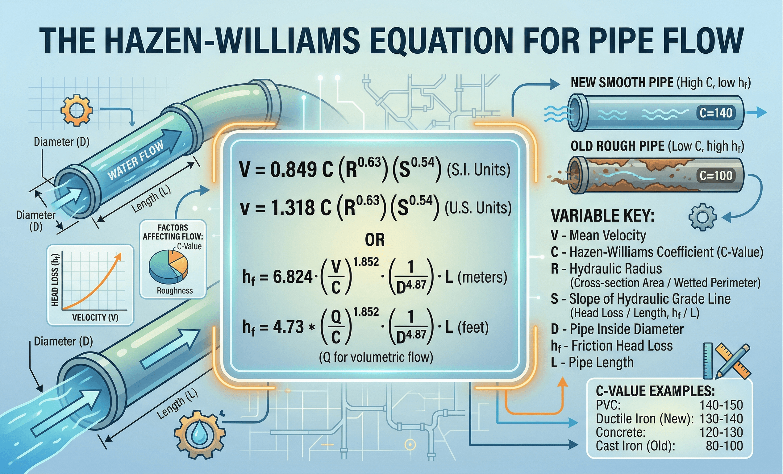
The Hazen-Williams equation is an empirical formula used to estimate friction head loss in full, pressurized water pipes carrying water.
Most readers want this first: Hazen-Williams is one of the fastest ways to estimate head loss in a full water pipe. Use the SI form with the 10.67 constant when flow is in m³/s and diameter is in m. Use a US customary form only when the matching units and constant are used consistently. For non-water fluids, unusual temperatures, or broader fluid analysis, Darcy-Weisbach is usually the better method.
The Hazen-Williams equation stays popular because it gives practical water-pipe friction-loss estimates without requiring viscosity, Reynolds number, or friction-factor iteration. That speed makes it useful in municipal water systems, domestic water piping, irrigation, and fire-protection layouts where engineers need a quick answer for head loss, flow capacity, or pipe diameter.
The tradeoff is that Hazen-Williams is not a universal pipe-flow equation. It is an empirical method intended for water in full, pressurized pipes and is best suited to turbulent conditions. When you move outside that use case, the formula becomes less reliable, which is why good design practice always starts by checking whether the method matches the system you are analyzing.
Editorial note: this page is written for practical engineering use. Hazen-Williams is convenient, but the result depends heavily on choosing a realistic \(C\) value, using the correct unit form, and confirming that the pipe is full and pressurized.
Hazen-Williams equation variables, units, and notation
The Hazen-Williams equation is simple to use only when the unit system is kept consistent from start to finish. The constant changes with the unit basis, so one of the most common calculation mistakes is mixing SI and US customary terms in the same equation.
Common notation
| Symbol | Meaning | Typical unit | What it represents |
|---|---|---|---|
| \(Q\) | flow rate | m³/s, L/s, ft³/s, gpm | The volumetric flow of water through the pipe. |
| \(d\) | inside pipe diameter | m, mm, ft, in | The internal flow diameter, not just the nominal pipe size on a catalog. |
| \(L\) | pipe length | m, ft | The hydraulic length of the pipe run being checked. |
| \(h_f\) | friction head loss | m, ft | The head lost due to pipe friction over the evaluated length. |
| \(S_f\) | friction slope | m/m or ft/ft | The head-loss gradient, equal to \(h_f/L\). |
| \(C\) | Hazen-Williams coefficient | dimensionless | An empirical roughness coefficient based on pipe material and condition. |
Unit and usage notes
- The SI form commonly uses \(S_f = 10.67\,Q^{1.852}/(C^{1.852}d^{4.87})\) with \(Q\) in m³/s and \(d\) in m.
- A common US customary full-pipe form uses \(S_f = 4.73\,Q^{1.852}/(C^{1.852}d^{4.87})\) with \(Q\) in ft³/s and \(d\) in ft.
- Fire-protection calculations may also use rearranged pressure-drop forms with different constants depending on whether flow is in gpm and diameter is in inches.
- Typical new plastic pipes often use \(C \approx 140\text{–}150\), while older, rougher, or more conservative assumptions use lower values.
- Minor losses from fittings, valves, meters, and bends are not included in the basic Hazen-Williams equation.
For direct solving and unit conversion, use the Hazen-Williams Calculator to estimate head loss, allowable flow, or required pipe diameter.
How the Hazen-Williams equation works in practice
The Hazen-Williams equation is a distributed-friction relationship. It predicts how much energy is lost to wall friction as water moves through a full pipe. The practical reason engineers like it is that it is fast. The practical reason engineers still have to be careful is that the result is highly sensitive to pipe diameter and reasonably sensitive to the selected \(C\) value.
Method 1: Solve for head loss when flow and diameter are known
This is the most common use case. You know the water flow rate, the pipe length, the inside diameter, and a reasonable Hazen-Williams coefficient. The goal is to estimate friction slope and total head loss so you can check pressure availability, pump demand, or whether a proposed line size is too restrictive.
This form is useful because it separates the slope from the total run length. In design practice, engineers often compare head loss per 100 m or per 100 ft between candidate diameters to decide whether a pipe size is balanced, oversized, or likely to create excess pressure loss.
Method 2: Rearrange the equation to solve for flow or diameter
Many real problems start with a design limit instead of a known flow. You may know the maximum allowable head loss, available pressure, or pressure budget and need to determine how much water the line can carry or what diameter is required.
Diameter has the strongest influence in the equation because it appears to the 4.87 power. That is why a modest increase in pipe size can sharply reduce friction losses. In actual design, this becomes a tradeoff between installation cost, available pressure, allowable velocity, and long-term operating performance.
The key limitation is that Hazen-Williams does not explicitly include viscosity or Reynolds number. That simplicity is what makes it convenient, but it is also why Darcy-Weisbach remains the more general and more widely applicable method for broader fluid systems.
Worked examples for the Hazen-Williams equation
These examples address the most common search intents: head loss for a known pipe, allowable flow for a design limit, and how the chosen \(C\) value changes the result.
Example 1: Head loss in a PVC water main
Scenario: Water flows at \(Q = 0.020\ \text{m}^3/\text{s}\) through a 150 mm internal diameter PVC pipe over a length of 250 m. Assume \(C = 145\). Estimate the friction slope and total head loss.
Steps:
- Convert the pipe diameter to metres so the SI form is consistent.
- Compute the friction slope using the SI constant 10.67.
- Multiply the slope by pipe length to get total head loss.
Result: the estimated friction slope is about 0.0129 m/m and the total friction head loss is about 3.23 m.
Interpretation: this is a practical water-distribution style result. The next engineering step is usually checking minor losses, elevation change, and whether the remaining pressure is still acceptable at the downstream point.
Example 2: Allowable flow for a head-loss limit
Scenario: A full pressurized water pipe has \(d = 0.20\ \text{m}\), \(L = 300\ \text{m}\), and \(C = 130\). The maximum allowable head loss is 4.5 m. Estimate the maximum flow rate.
Steps:
- Convert total allowable head loss into a friction slope.
- Insert the diameter, \(C\), and friction slope into the rearranged flow equation.
- Solve for \(Q\) and then check whether the resulting velocity is reasonable.
Result: the estimated allowable flow is about 0.041 m³/s, or about 41 L/s.
Interpretation: this is a useful quick sizing check, but a final design should still verify velocity criteria, minor losses, and project-specific code requirements.
Example 3: How changing the Hazen-Williams coefficient affects head loss
Scenario: A designer compares two water lines with the same length, diameter, and flow, but one uses \(C = 150\) and the other uses \(C = 100\). How does the head-loss ratio change?
Steps:
- Hold flow, diameter, and length constant.
- Use the inverse \(C^{1.852}\) relationship.
- Compute the head-loss ratio between the rougher and smoother pipe conditions.
Result: the line with \(C = 100\) has about 2.12 times the friction head loss of the line with \(C = 150\).
Interpretation: this is why a careless \(C\) assumption can distort design output. Pipe condition, aging, scale buildup, and conservative design choices materially change the result.
Common mistakes, assumptions, and engineering checks
Hazen-Williams is fast enough to encourage shortcut thinking. That is exactly why the best use of the equation is inside a broader design workflow that checks applicability, selected \(C\) value, minor losses, and whether a different equation should be used instead.
The Hazen-Williams equation is intended for full, pressurized water pipes in turbulent conditions. It is not a universal friction-loss model for every pipe and every fluid.
- Do not use it for oils, chemicals, slurries, or highly viscous liquids.
- Do not use it for open channels or partially full pipes.
- Use Darcy-Weisbach when viscosity, Reynolds number, or non-water fluids matter directly.
The Hazen-Williams coefficient is often the most judgment-based input in the whole problem. A value that is too optimistic can make a pipe appear to perform better than it will in service, especially in older systems.
- Use new-pipe values only when that assumption is justified.
- Use lower \(C\) values for conservative checks or aging-system evaluations when appropriate.
- Document the basis for the selected coefficient in your design record.
Hazen-Williams covers distributed friction along the pipe run. Real systems also lose energy through fittings, valves, bends, tees, strainers, meters, entrances, and exits.
- Add minor losses separately using equivalent length or loss coefficients.
- Check velocity along with head loss, especially in domestic water and fire systems.
- Compare the final result with a Bernoulli-style energy balance when available pressure is critical.
Hazen-Williams Equation FAQ
What is the Hazen-Williams equation used for?
It is used to estimate friction head loss, flow rate, or required pipe diameter in full, pressurized water pipes. It is especially common in potable water, municipal distribution, and fire-protection piping.
When should I use Hazen-Williams instead of Darcy-Weisbach?
Use Hazen-Williams when you need a fast empirical estimate for water in full, pressurized turbulent flow. Use Darcy-Weisbach when fluid properties, viscosity effects, laminar flow, or non-water fluids matter more directly.
What does the Hazen-Williams coefficient \(C\) mean?
\(C\) is an empirical roughness coefficient that reflects pipe material and condition. Higher \(C\) values represent smoother pipes and lower predicted head loss for the same flow and diameter.
Does Hazen-Williams include losses from fittings and valves?
No. The basic equation accounts for distributed friction along the pipe only. Minor losses from fittings, valves, bends, and other components must be added separately.
References and further reading
- Hazen-Williams Water Flow Formula | Engineering ToolBox – practical reference for common forms of the equation and unit-system constants.
- Hazen-Williams Equation | LMNO Engineering – useful worked forms and engineering notes for solving common pipe-flow variables.
- Hazen-Williams Calculator | Turn2Engineering – direct solve mode for head loss, flow, and diameter with water-system design context.
- Bernoulli Equation Calculator | Turn2Engineering – useful next step for combining head loss with pressure, velocity, and elevation analysis.