Key Takeaways
- Definition: Fourier’s Law relates conductive heat transfer to a material’s thermal conductivity, flow area, and temperature gradient.
- Main use: Engineers use it to estimate heat loss or heat gain through walls, insulation, pipes, components, and equipment surfaces.
- Watch for: The common algebraic form assumes steady, one-dimensional conduction with constant \(k\) and no internal heat generation.
- Outcome: You will be able to select the right form, solve for heat rate or thickness, and check whether the result is physically reasonable.
Table of Contents
Heat flows across a wall from the hot side to the cold side
Fourier’s Law describes conduction by relating heat flow to thermal conductivity, cross-sectional area, and the temperature gradient through a material.
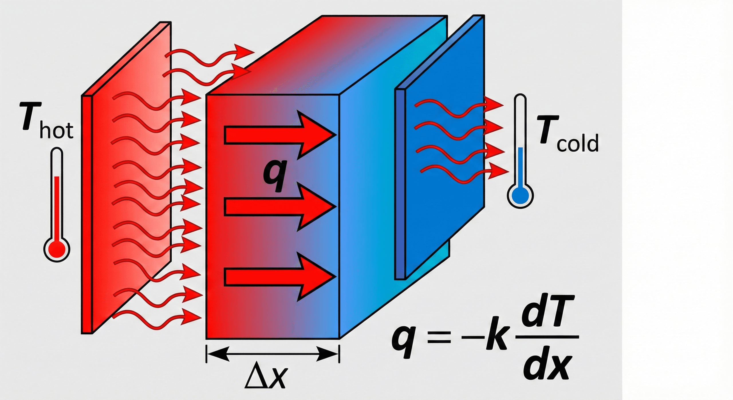
The key thing to notice is direction: heat moves from the hotter face toward the colder face. The steeper the temperature drop over the thickness, and the more conductive the material, the larger the heat transfer rate becomes.
What is Fourier’s Law?
Fourier’s Law is the foundational equation for conduction heat transfer. It states that heat flows through a material in response to a temperature gradient, and the rate of that heat flow depends on the material property called thermal conductivity.
In practical engineering terms, this is the equation you reach for when you need to estimate how much heat passes through a wall, insulation layer, metal plate, pipe wall, or equipment housing. It is also the starting point for more advanced heat-transfer work involving composite walls, thermal resistance networks, transient conduction, or multi-dimensional conduction models.
The real problem most readers are trying to solve is usually one of these: How much heat is leaking through this layer? How thick does the insulation need to be? Why is this component running hotter than expected? Fourier’s Law is the first equation that anchors those decisions.
The Fourier’s Law formula
The most general one-dimensional differential form of Fourier’s Law is:
If you want heat flux instead of total heat rate, divide by area:
For the common engineering case of steady, one-dimensional conduction through a flat wall of thickness \(L\) with constant thermal conductivity, the equation becomes:
The negative sign in the differential form is important. It reminds you that heat flows down the temperature gradient, from higher temperature toward lower temperature. In the algebraic flat-wall form, that direction is usually handled by defining \(T_H\) as the hot-side temperature and \(T_C\) as the cold-side temperature.
Variables and units
To use Fourier’s Law correctly, you need to distinguish between total heat rate and heat flux, and you need to keep thermal conductivity and length units fully consistent.
- \(q\) or \(q_x\) Total heat transfer rate through the surface. Typical SI unit: W. Typical US customary unit: BTU/hr.
- \(q”\) Heat flux, or heat transfer rate per unit area. Typical SI unit: W/m\(^2\). Typical US customary unit: BTU/(hr·ft\(^2\)).
- \(k\) Thermal conductivity, a material property that measures how easily heat conducts. Typical SI unit: W/(m·K). Typical US customary unit: BTU/(hr·ft·°F).
- \(A\) Area normal to the heat-flow direction. Typical SI unit: m\(^2\). Typical US customary unit: ft\(^2\).
- \(\frac{dT}{dx}\) Temperature gradient through the material. Typical SI unit: K/m or °C/m.
- \(L\) Conduction path length or wall thickness. Typical SI unit: m. Typical US customary unit: ft or in, after proper conversion.
A temperature difference in kelvins is numerically the same as a difference in degrees Celsius, but the same is not true when converting to or from Fahrenheit-based conductivity units.
For a fixed material, area, and temperature difference, doubling the wall thickness should roughly cut the steady conductive heat rate in half.
| Variable | Meaning | SI units | US customary units | Typical range | Notes |
|---|---|---|---|---|---|
| \(k\) | Thermal conductivity | W/(m·K) | BTU/(hr·ft·°F) | Very low for insulation, high for metals | Usually temperature-dependent in real materials. |
| \(A\) | Heat-transfer area | m\(^2\) | ft\(^2\) | Project-dependent | Use the area actually normal to conduction. |
| \(L\) | Thickness / path length | m | ft, in | Project-dependent | Thicker layers reduce heat transfer. |
| \(\Delta T\) | Temperature difference | K or °C difference | °F difference | Project-dependent | Use a temperature difference, not absolute values, in the flat-wall form. |
How to rearrange Fourier’s Law
Engineers often rearrange Fourier’s Law to solve for thickness, conductivity, or allowable temperature difference. The most common steady flat-wall solve-for forms are:
After rearranging, make sure the trend still makes physical sense. Higher \(k\) or larger area should increase heat transfer, while greater thickness should reduce it in the steady flat-wall case.
Where engineers use this equation
Fourier’s Law is used anywhere conduction matters enough to affect performance, energy loss, safety, comfort, or equipment life. It appears in building envelopes, process equipment, electronics cooling, insulation design, and thermal component checks.
- Building and envelope design: estimating heat loss through walls, roofs, doors, insulation, and thermal layers.
- Mechanical and process equipment: evaluating heat transfer through tanks, pipes, exchangers, linings, and insulated surfaces.
- Electronics and thermal management: checking whether chips, heat spreaders, base plates, or housings can conduct heat away fast enough.
- Materials and component design: comparing materials based on conductivity and selecting thicknesses that hit thermal limits.
In practice, Fourier’s Law is often paired with heat-transfer fundamentals, resistance methods, or calculator tools such as the Thermal Conductivity Calculator and the Heat Transfer Calculator.
Worked example
Example problem
A flat wall has area \(A = 12 \,\text{m}^2\), thickness \(L = 0.20 \,\text{m}\), and thermal conductivity \(k = 0.80 \,\text{W/(m·K)}\). The hot-side surface is at \(35^\circ\text{C}\) and the cold-side surface is at \(5^\circ\text{C}\). Estimate the steady conductive heat transfer rate through the wall.
First identify the temperature difference:
Now apply the steady flat-wall form of Fourier’s Law:
Carrying out the arithmetic:
The wall conducts heat at about 1.44 kW from the warm side to the cold side. That is a useful design number because it tells you the scale of heating or cooling load associated with this layer alone.
If that answer feels too large, notice what is driving it: a fairly large area, a noticeable temperature difference, and only moderate thickness. Increasing thickness or switching to a lower-\(k\) insulation layer would reduce the heat loss directly.
Assumptions behind the equation
Fourier’s Law is always grounded in conduction physics, but the simplified algebraic form used in hand calculations depends on several assumptions that are easy to overlook.
- 1 Heat transfer is conduction-dominated through the material of interest.
- 2 For \( q = kA\Delta T/L \), the process is steady and one-dimensional.
- 3 Thermal conductivity is approximately constant across the temperature range used.
- 4 There is no internal heat generation within the layer being modeled.
- 5 The area and thickness represent the real conduction path, not an oversimplified geometry.
Neglected factors
Basic Fourier’s Law calculations do not automatically capture convection on the surfaces, radiative exchange, contact resistance, multidimensional edge effects, thermal bridges, temperature-dependent conductivity, or transient thermal storage.
- Convection and radiation: matter when the thermal bottleneck is at the surface rather than in the solid layer.
- Composite layers: matter when multiple materials sit in series and you need total thermal resistance.
- Transient effects: matter when temperatures are changing with time and the system has not reached steady state.
Engineering judgment and field reality
In real projects, the equation is often the easy part. The hard part is knowing whether the temperatures, material property, thickness, and actual conduction path reflect what is happening on site or in the hardware.
Installed insulation can be compressed, wet, discontinuous, or bridged by fasteners and framing. In equipment, thermal contact resistance or imperfect mating surfaces can dominate the heat path even when the solid material conductivity looks excellent on paper.
If a simple Fourier’s Law check gives an unrealistically low heat loss, ask whether you have ignored a surface film, a thermal bridge, or a gap that changes the real heat-transfer path.
When this equation breaks down
Fourier’s Law remains the foundation of conduction analysis, but the simplest forms stop being reliable when the physics become more complicated than steady one-dimensional conduction through a uniform layer.
Do not trust the simple flat-wall form blindly when conductivity varies strongly with temperature, geometry forces radial or multidimensional heat flow, internal heat generation exists, or transient behavior matters.
At very small scales, in highly anisotropic materials, or in problems dominated by convection or radiation rather than conduction, you need a broader heat-transfer model rather than a single algebraic conduction shortcut.
Fourier’s Law vs. related equations
Fourier’s Law is one piece of the heat-transfer toolkit. It answers the conduction part of the problem, but engineers often need to compare it with neighboring methods and quantities.
| Equation / method | Best used for | Key assumption | Main limitation |
|---|---|---|---|
| Fourier’s Law | Conduction through solids or stationary layers | Heat flow follows a temperature gradient through a material | Does not by itself capture convection, radiation, or full thermal networks |
| Thermal resistance method | Multi-layer walls and combined conduction paths | Individual resistances can be represented and summed | Still depends on correct boundary conditions and material data |
| Newton’s Law of Cooling | Convection at surfaces | Uses a heat-transfer coefficient \(h\) | Applies to fluid-side surface exchange, not solid conduction through a wall |
| Heat equation / transient conduction | Temperature changing with time inside a body | Thermal storage matters | Requires more data and a time-dependent model |
Common mistakes and engineering checks
- Using the flat-wall form for cylindrical or spherical conduction without adjusting the geometry.
- Forgetting that \(k\) may vary with temperature or moisture content.
- Mixing W/(m·K) with inch- or foot-based geometry without proper conversion.
- Using surface temperatures interchangeably with surrounding fluid temperatures.
- Ignoring convection or contact resistance and blaming the material instead.
Ask whether the result scales correctly. Larger \(A\), larger \(\Delta T\), or larger \(k\) should increase heat transfer, while larger \(L\) should reduce it in the simple steady model.
| Check item | What to verify | Why it matters |
|---|---|---|
| Units | Conductivity, area, thickness, and temperature difference are all in a consistent system. | Mixed-unit conduction calculations can look clean but still be completely wrong. |
| Geometry | The chosen area and thickness match the actual heat-flow direction. | Wrong geometry means the model no longer represents the physical path. |
| Magnitude | The heat rate feels reasonable compared with insulation level and temperature difference. | Outlier results often signal a bad \(k\) value, wrong thickness, or missed resistance. |
Frequently asked questions
Fourier’s Law describes conductive heat transfer. It relates heat flow to thermal conductivity, area, and temperature gradient, showing that heat moves from hotter regions to colder regions.
The negative sign shows direction. Heat flows opposite the direction of increasing temperature, so conductive heat transfer moves down the temperature gradient.
The flat-wall form \( q = kA\Delta T/L \) is used for steady, one-dimensional conduction through a layer of uniform thickness and constant thermal conductivity with no internal heat generation.
Heat rate is the total heat transfer, usually in watts or BTU/hr. Heat flux is heat transfer per unit area, usually in W/m\(^2\) or BTU/(hr·ft\(^2\)).
Summary and next steps
Fourier’s Law is the core equation for conduction. It connects heat transfer to thermal conductivity, area, and the temperature gradient, giving engineers a practical way to estimate thermal losses and size materials.
The most important judgment step is matching the equation form to the real physics. The common flat-wall expression is powerful, but only when steady, one-dimensional conduction is a fair approximation.
Where to go next
Continue your learning path with these curated next steps.
-
Prerequisite: Heat Transfer
Build the broader foundation behind conduction, convection, and radiation before moving deeper into applied thermal design.
-
Current topic: Fourier’s Law
Use this page as your quick-reference source for the equation, units, assumptions, and worked-example logic.
-
Advanced: Heat Transfer Calculator
Move from the formula itself into applied sizing of heat loss and required insulation thickness.