Key Takeaways
- Definition: The thermal expansion equation estimates how much a material expands or contracts when its temperature changes.
- Main use: Engineers use it to check movement allowances, gaps, tolerances, pipe runs, frames, rails, panels, and assemblies exposed to temperature swings.
- Watch for: The simple equation predicts free expansion; restrained expansion can create thermal stress instead of visible movement.
- Outcome: After reading, you can choose the correct form, use consistent units, solve for unknowns, and judge whether the answer is realistic.
Table of Contents
Thermal expansion shows material growth as temperature rises
The thermal expansion equation relates temperature change to dimensional change, letting engineers estimate how much a material grows or shrinks.
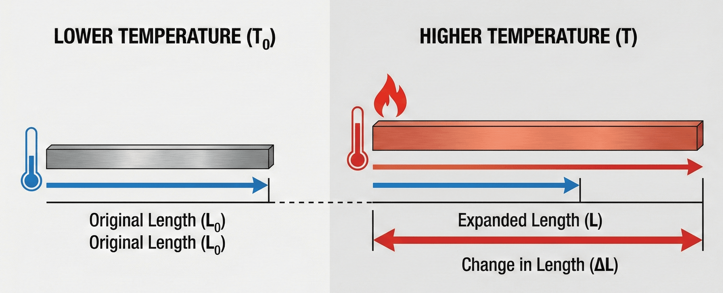
The first thing to notice is that the expansion is proportional to the starting length. A long member and a short member made of the same material may experience the same temperature change, but the longer member moves more because the original dimension is larger.
What is the thermal expansion equation?
The thermal expansion equation is a material-response equation used to estimate dimensional change caused by a temperature change. In its most common engineering form, it calculates the change in length of a solid member using the material’s coefficient of linear thermal expansion, the original length, and the temperature difference.
The real engineering problem is usually not “what is the formula?” It is whether a beam, pipe, rail, panel, shaft, bracket, or enclosure has enough room to move without binding, cracking, buckling, leaking, or forcing unwanted stress into connected parts.
For quick calculations, the linear form is the most common starting point. Area and volume expansion forms are used when surface area or volume change matters, such as tank contents, solid blocks, thermal fits, enclosures, or approximate volumetric material growth.
The thermal expansion equation formula
The primary equation for linear thermal expansion is:
This form says the change in length \(\Delta L\) increases when the coefficient of thermal expansion \(\alpha\), original length \(L_0\), or temperature change \(\Delta T\) increases. The equation assumes the material is free to expand and that \(\alpha\) is approximately constant over the temperature range.
For many isotropic solids, area and volume expansion can be approximated from the same linear coefficient:
The factors \(2\alpha\) and \(3\alpha\) are approximations for isotropic materials where expansion is similar in all directions. If a material expands differently by direction, such as some composites, woods, crystals, or layered materials, use direction-specific expansion data instead of assuming one coefficient applies everywhere.
Variables and units
Thermal expansion calculations are usually simple, but unit consistency matters. The coefficient of thermal expansion must match the temperature-difference unit, and the output dimension will use the same length unit as the original dimension.
- \(\Delta L\) Change in length, typically in m, mm, ft, or in. Positive means expansion; negative means contraction.
- \(\alpha\) Coefficient of linear thermal expansion, usually in \(1/K\), \(1/^\circ C\), or \(1/^\circ F\).
- \(L_0\) Original length before the temperature change, using the same length system desired for the result.
- \(\Delta T\) Temperature change, equal to final temperature minus initial temperature.
- \(\Delta A,\Delta V\) Change in area or volume when surface or volumetric expansion is being approximated.
A temperature difference of \(1~K\) equals a temperature difference of \(1^\circ C\), so coefficients in \(1/K\) and \(1/^\circ C\) are numerically compatible for \(\Delta T\). Do not mix coefficients based on Fahrenheit with Celsius or Kelvin temperature differences unless you convert the coefficient.
| Variable | Meaning | SI units | US customary units | Practical note |
|---|---|---|---|---|
| \(\Delta L\) | Length change | m, mm | ft, in | Use the same length unit as \(L_0\). |
| \(\alpha\) | Linear thermal expansion coefficient | \(1/K\) or \(1/^\circ C\) | \(1/^\circ F\) | Material property; use project-specific or datasheet values when available. |
| \(L_0\) | Original length | m, mm | ft, in | Use the actual free length that can expand, not always the full part length. |
| \(\Delta T\) | Temperature change | K or \(^{\circ}C\) difference | \(^{\circ}F\) difference | Use temperature difference, not absolute temperature. |
Many metals have linear expansion coefficients on the order of \(10^{-6}\) to \(25 \times 10^{-6}/K\). Plastics can be much higher. If your result suggests centimeters of movement over a short metal part under a modest temperature swing, check the coefficient units first.
How to rearrange the thermal expansion equation
Engineers often rearrange the thermal expansion equation when they know allowable movement, available gap, or observed movement and need to solve backward for temperature change, required length, or a material property.
Use this form when measured expansion is known and you want to estimate or verify the coefficient of thermal expansion.
Use this form when a gap, tolerance, or field-measured displacement is known and you want the temperature change that would produce it.
Use this form to estimate the length of member that would create a known amount of free thermal movement under a specified temperature swing.
After rearranging, verify that the units collapse correctly. For example, \(\alpha L_0 \Delta T\) should leave only length because \(1/K\) multiplied by \(K\) is dimensionless.
Worked example
Steel beam expansion under a daily temperature swing
Suppose a steel beam is \(10~m\) long at its reference temperature. The expected temperature increase is \(35^\circ C\), and the steel coefficient of linear thermal expansion is \(12 \times 10^{-6}/^\circ C\). Estimate the free expansion.
The degrees Celsius difference cancels the inverse degrees Celsius in the coefficient. The result remains in meters because the original length was entered in meters.
The beam would expand by about \(4.2~mm\) if it were free to move. In a real connection, that movement may be absorbed by a slotted hole, expansion joint, flexible support, bearing detail, or clearance gap.
A few millimeters may sound small, but it can matter in bolted connections, façade panels, bridge joints, rails, piping supports, precision assemblies, and parts with tight tolerances.
Where engineers use the thermal expansion equation
Thermal expansion matters whenever temperature changes are large enough to affect fit, clearance, alignment, or stress. The equation is often used early in design because it quickly shows whether movement must be intentionally accommodated.
- Structural engineering: estimating bridge deck movement, façade panel expansion, rail expansion, bearing movement, and expansion joint demand.
- Mechanical engineering: checking shaft fits, sleeves, housings, machine frames, thermal clearances, and interference fits.
- Piping and HVAC: estimating pipe growth so loops, guides, anchors, and supports can accommodate thermal movement.
- Electrical and electronics: evaluating enclosure movement, conductor sag, printed circuit board mismatch, and thermal cycling effects.
- Materials and manufacturing: assessing tolerance stackups when parts are assembled or operated at different temperatures.
If the part is free to move, calculate \(\Delta L\). If the part is restrained, also evaluate thermal stress. If two bonded materials expand differently, check differential expansion rather than treating the assembly as one uniform material.
Assumptions behind the equation
The simple thermal expansion equation is powerful because it is fast, but it depends on several assumptions. These assumptions are usually reasonable for first-pass calculations, but they should be checked before using the result for a final design decision.
- 1 The material is free to expand or contract without significant restraint.
- 2 The coefficient of thermal expansion is approximately constant over the temperature range.
- 3 The temperature change is reasonably uniform through the part being evaluated.
- 4 The material behaves approximately isotropically if area or volume expansion is estimated from \(\alpha\).
Neglected factors
The basic equation does not automatically include stress, creep, temperature gradients, nonlinear material behavior, plastic deformation, connection stiffness, or construction tolerances.
- Restraint: blocked expansion can create thermal stress instead of visible movement.
- Temperature gradients: one side heating more than another can create bending, warping, or curvature.
- Material mismatch: bonded materials with different coefficients can create differential movement and interface stresses.
- Large temperature ranges: \(\alpha\) may vary enough with temperature that a constant value becomes too approximate.
Engineering judgment and field reality
In the field, thermal movement rarely happens in a perfectly clean textbook way. Parts are connected, supports have friction, bolts clamp surfaces together, seals age, slots may not be centered, and actual temperatures may differ from ambient air readings.
The free-expansion result is often best treated as the movement demand. The design question is then whether the connection, joint, support, or clearance detail can safely absorb that demand without creating damage or serviceability problems.
Do not use only the average air temperature if the component is exposed to solar radiation, process heat, hot fluids, cold starts, or enclosure effects. The material temperature can be meaningfully different from the surrounding air.
When the thermal expansion equation breaks down
The simple equation becomes less reliable when the real system is dominated by restraint, nonuniform heating, complex material behavior, or direction-dependent expansion. In those cases, the equation may still provide a useful estimate, but it should not be the only design check.
If expansion is restrained, do not stop at \(\Delta L = \alpha L_0 \Delta T\). The critical issue may be thermal stress, buckling, bearing pressure, seal compression, or connection force rather than visible movement.
| Situation | Why the simple equation may fail | Better next check |
|---|---|---|
| Restrained member | Expansion is blocked, so stress can build up. | Thermal stress and support reaction analysis. |
| Composite or layered material | Expansion may differ by direction or layer. | Differential expansion and compatibility checks. |
| Large temperature swing | \(\alpha\) may not remain constant. | Temperature-dependent material data. |
| Nonuniform heating | Gradients can cause bending or warping. | Thermal gradient or finite element analysis. |
Common mistakes and engineering checks
Most thermal expansion errors come from unit mismatch, using the wrong length, ignoring restraint, or assuming the part temperature equals the room temperature. A quick check before accepting the result can prevent large design mistakes.
- Using the wrong coefficient: \(1/^\circ F\) and \(1/^\circ C\) coefficients are not numerically interchangeable.
- Using total temperature instead of temperature change: the equation needs \(\Delta T\), not the final temperature alone.
- Using the wrong length: use the free expanding length, span, run, or segment that actually contributes to movement.
- Ignoring sign: positive \(\Delta T\) expands most materials; negative \(\Delta T\) contracts them.
- Forgetting restraint: a restrained component may produce force instead of movement.
For a typical metal member, expect small but not zero movement: millimeters over meter-scale lengths for moderate temperature changes. If the answer is orders of magnitude larger, recheck coefficient units and length units.
| Check item | What to verify | Why it matters |
|---|---|---|
| Temperature basis | Use \(\Delta T = T_f – T_i\). | The equation is based on temperature change, not absolute temperature. |
| Coefficient unit | Match \(1/K\), \(1/^\circ C\), or \(1/^\circ F\) to the temperature difference. | Coefficient mismatch can create a large numerical error. |
| Movement path | Confirm the member can actually expand freely. | Blocked movement can shift the problem from displacement to stress. |
| Material temperature | Use the component temperature, not just ambient air temperature. | Solar, process, and enclosure effects can change actual material temperature. |
Frequently asked questions
The thermal expansion equation calculates how much a material changes length, area, or volume when its temperature changes. The most common form is the linear equation \(\Delta L = \alpha L_0 \Delta T\).
Use consistent units. Length can be meters, millimeters, feet, or inches, but the result will follow that same length unit. The coefficient must match the temperature difference unit, such as \(1/K\), \(1/^\circ C\), or \(1/^\circ F\).
For linear expansion, rearrange \(\Delta L = \alpha L_0 \Delta T\) into \(\Delta T = \Delta L / (\alpha L_0)\). This is useful when allowable movement or observed movement is known.
Linear expansion estimates change in one dimension, area expansion estimates change in surface area, and volume expansion estimates change in three-dimensional volume. For isotropic solids, area expansion is often approximated with \(2\alpha\), and volume expansion with \(3\alpha\).
It becomes less reliable when temperature changes are very large, expansion is restrained, material properties vary strongly with temperature, heating is nonuniform, or the material expands differently in different directions.
Summary and next steps
The thermal expansion equation connects dimensional change to material coefficient, original dimension, and temperature change. The linear form \(\Delta L = \alpha L_0 \Delta T\) is the most common engineering version because it directly answers how much a member grows or shrinks under a temperature swing.
The most important judgment step is deciding whether the component is actually free to expand. If it is restrained, the calculation may need to move from displacement to thermal stress, support force, buckling risk, or connection detailing.
Where to go next
Continue your learning path with these curated next steps.
-
Prerequisite: Heat Transfer
Build the broader foundation behind temperature differences, thermal energy movement, and material response.
-
Current topic: Thermal Expansion Equation
Use this page as the quick-reference source for the equation, units, assumptions, and worked-example logic.
-
Advanced: Fourier’s Law
Learn how temperature gradients drive heat conduction, often creating the temperature conditions that lead to thermal expansion.