Key Takeaways
- Definition: The acceleration formula relates change in velocity to elapsed time, telling you how quickly motion speeds up, slows down, or reverses direction.
- Main use: Engineers use it for launch, braking, conveyors, elevators, motion-control profiles, and first-pass kinematics checks.
- Watch for: Unit consistency, sign convention, and whether constant acceleration is a valid assumption matter more than the algebra.
- Outcome: After reading, you should be able to solve for acceleration, time, or velocity change and judge whether the result is reasonable.
Table of Contents
Velocity Change Over Time Diagram
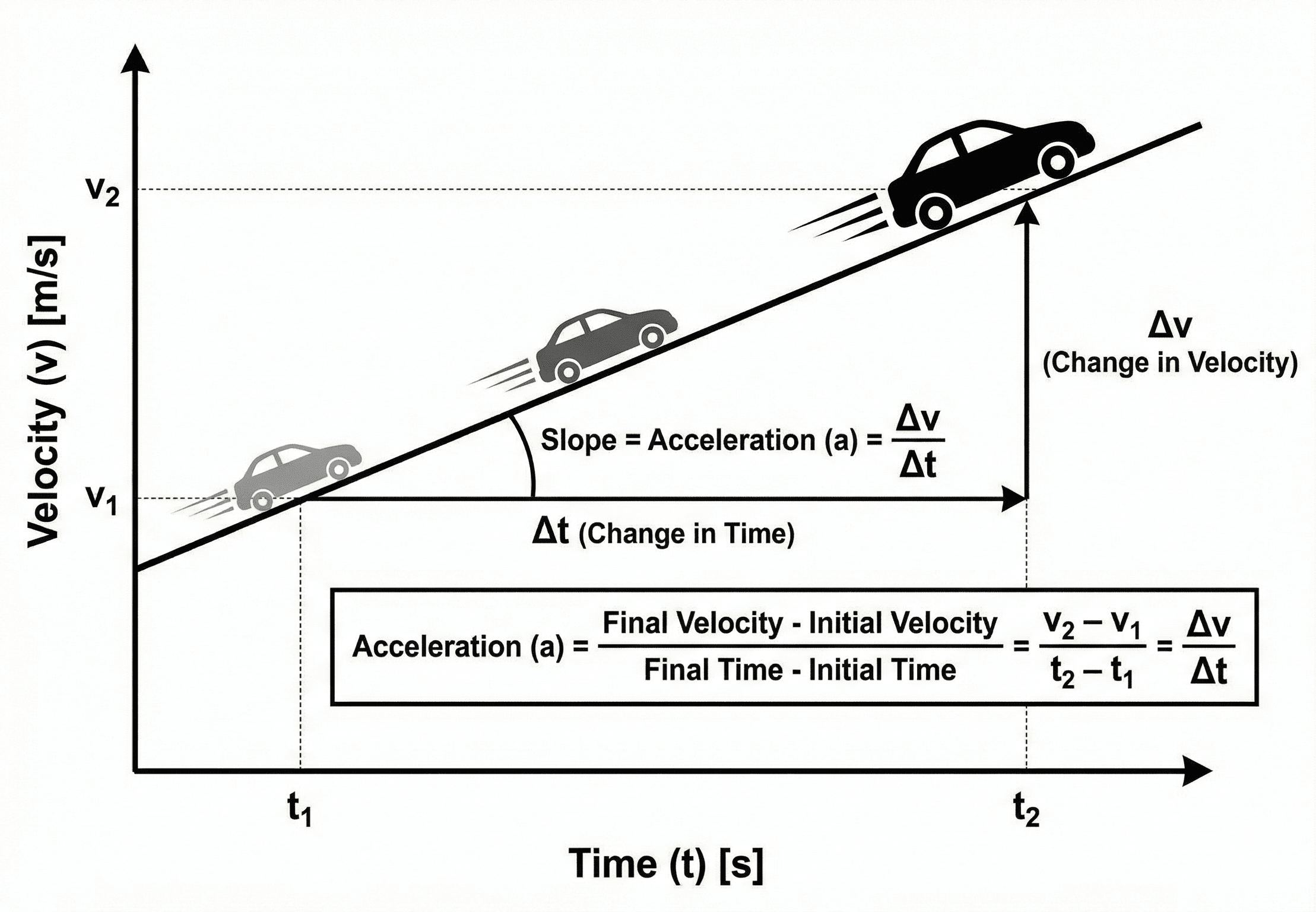
Notice first that acceleration is not just “speeding up.” It is the rate of velocity change. That means the sign matters, and the same equation can describe acceleration, braking, or motion in the opposite direction.
What is the Acceleration Formula?
The acceleration formula tells you how quickly velocity changes over time. In one-dimensional motion, it is one of the fastest ways to turn measured motion into a design-useful number, because it converts a change in speed and direction into an acceleration value you can compare against performance, safety, or comfort limits.
In practical engineering work, this equation appears in vehicle launch and braking checks, lift and conveyor motion profiles, actuator sizing, robotics timing, and first-pass kinematics problems. It is also the bridge between motion measurements and force calculations, because once acceleration is known, you can connect it to mass through Newton’s Second Law.
The Acceleration Formula
For average acceleration over a time interval, the most important form is the direct change-in-velocity relationship:
This equation says acceleration is the slope of velocity versus time. A steeper slope means a larger magnitude of acceleration. A flat line means zero acceleration. A downward slope means the acceleration is negative in the chosen positive direction.
The differential form above is the more general definition of instantaneous acceleration. For most hand calculations, exam problems, and first-pass engineering checks, the average form is what readers need first. When acceleration is assumed constant, it also connects directly to the standard kinematics relationships:
Variables and Units
The equation itself is simple, but mistakes usually come from symbols, signs, and units. Choose a positive direction first, keep that convention for every term, and convert all speeds and times into a consistent unit system before solving.
- \(a\) Acceleration. In SI this is usually m/s². In US customary work it is often ft/s², and some applications compare magnitude to \(g\).
- \(v\) Final velocity at the end of the interval. Keep its sign consistent with your chosen reference direction.
- \(v_0\) Initial velocity at the start of the interval. This is the reference motion before the change begins.
- \(\Delta v\) Change in velocity, defined as \(v-v_0\). This includes sign, so braking or reversal can produce a negative value.
- \(t,\ \Delta t\) Elapsed time over which the velocity change occurs. Time must be positive and in the same unit system as the velocity conversion.
If velocity is in m/s and time is in s, acceleration comes out in m/s². If you start with mph or km/h, convert velocity first instead of mixing transport units directly into the equation.
Everyday machine and vehicle accelerations are often on the order of a few m/s². If your answer is tens or hundreds of m/s² for a comfort-limited system, double-check the inputs and units.
| Variable | Meaning | SI units | US customary units | Typical range | Notes |
|---|---|---|---|---|---|
| \(a\) | Acceleration | m/s² | ft/s² | ~0 to 10+ for many common systems | Negative does not always mean slowing down; it means acceleration acts in the negative direction. |
| \(v,\ v_0\) | Final and initial velocity | m/s | ft/s | Application-dependent | Use signed velocities, not just magnitudes, when direction matters. |
| \(\Delta t\) | Elapsed time | s | s | Fractions of a second to minutes | Average acceleration becomes less descriptive as the interval gets longer and motion becomes less uniform. |
How to Rearrange the Acceleration Formula
Engineers often do not solve for acceleration directly. Just as often, they solve for time required to reach a target speed or for the final velocity after a known acceleration interval. Starting from \(a=\dfrac{v-v_0}{t}\), the most useful rearrangements are:
When distance is known but time is not, the most useful companion form is not another direct rearrangement of the average formula. Instead, move to the constant-acceleration equation:
After rearranging, check dimensions. Time should reduce to seconds, velocity to m/s or ft/s, and acceleration to m/s² or ft/s². If units do not collapse correctly, the algebra or conversion likely went wrong.
Where Engineers Use This Equation
The acceleration formula is a foundational motion equation, but its value comes from how often it appears in real systems:
- Vehicles and transportation: estimating launch performance, stopping rates, merge timing, and ride-quality limits.
- Elevators, lifts, and material handling: checking whether motion is smooth enough for passengers or product stability.
- Robotics and automation: sizing motion profiles for actuators, gantries, pick-and-place systems, and conveyor transitions.
- Safety and comfort review: comparing acceleration magnitude against allowable user experience or load-protection thresholds.
In early design work, acceleration is often the motion metric that reveals whether a concept feels realistic before you move into detailed force, power, or controls analysis.
Worked Example
Example problem — conveyor ramp-up for packaged product
A packaging conveyor starts from rest and reaches \(1.8\ \text{m/s}\) in \(3.0\ \text{s}\). Assume the ramp-up is approximately constant acceleration. Find the average acceleration, then estimate the distance traveled during the ramp-up.
The average acceleration is \(0.60\ \text{m/s}^2\). Because the problem states a constant ramp-up, you can now use the constant-acceleration displacement relationship:
So the conveyor travels 2.7 m during the ramp-up phase. That number helps with product spacing, guard placement, and downstream timing logic.
The answer is reasonable because the acceleration is modest and the ramp distance is large enough to avoid a harsh motion jump. If the same speed change happened in 0.3 s instead of 3.0 s, the result would be ten times larger and likely too abrupt for many conveyor or passenger-facing systems.
Assumptions and Limits Behind the Equation
The direct average-acceleration formula is always mathematically valid over a chosen interval, but its usefulness depends on what you are trying to represent physically. Once you start using companion kinematics equations, the assumptions become much more important.
- 1 Motion is being interpreted along a clearly defined direction or axis.
- 2 Velocities and time are measured consistently in one unit system.
- 3 If you use \(v=v_0+at\) or distance-based forms, acceleration is assumed approximately constant during the interval.
Neglected factors
The simple form hides several effects that can matter in real projects:
- Jerk: how fast acceleration itself changes. This matters in ride comfort, servo motion, and fragile-product handling.
- Drag and resistance: aerodynamic drag, friction, rolling resistance, or fluid resistance can make acceleration vary with speed.
- Traction or control limits: tire grip, actuator saturation, motor torque curves, or controller tuning may cap the achievable acceleration.
- Curved motion: turning systems require centripetal acceleration analysis in addition to straight-line tangential acceleration.
Do not rely on constant-acceleration motion formulas when the system is clearly driven by changing force, varying drag, or multi-stage control logic. In that case, use measured data, numerical integration, or a more complete dynamic model.
Common Mistakes and Engineering Checks
- Using km/h, mph, and seconds together without converting velocity first.
- Dropping the sign on velocity change and reporting only magnitude.
- Using the time-based form when time is unknown but distance is known.
- Assuming constant acceleration even though the system is clearly speed-dependent or controller-limited.
- Stopping at the arithmetic result without asking whether the number makes physical sense.
Ask two quick questions: does the sign match the motion direction, and is the magnitude believable for the system? A passenger elevator, for example, should not show race-car-like acceleration values.
| Check item | What to verify | Why it matters |
|---|---|---|
| Units | Velocity and time are in a compatible system before substitution. | Bad conversions are one of the fastest ways to produce nonsense acceleration values. |
| Magnitude | The result is plausible for the machine, vehicle, or person involved. | A wildly large value often means the interval, assumption, or input data is wrong. |
| Sign convention | Positive and negative directions stayed consistent from start to finish. | The sign is part of the physical meaning, not just a math detail. |
Frequently Asked Questions
The acceleration formula is \(a=\dfrac{\Delta v}{\Delta t}\), meaning acceleration equals the change in velocity divided by the elapsed time.
In SI, acceleration is usually written in m/s². In US customary work, ft/s² is common. The important rule is to keep velocity and time in a consistent unit system before solving.
Starting from \(a=\dfrac{v-v_0}{t}\), solve for time as \(t=\dfrac{v-v_0}{a}\), as long as the acceleration is not zero.
Average acceleration uses a finite interval, \(\dfrac{\Delta v}{\Delta t}\). Instantaneous acceleration describes the rate of change at a specific moment and is written as \(\dfrac{dv}{dt}\).
It stops being enough when acceleration changes significantly over time, when drag or traction makes motion nonlinear, when jerk matters, or when the motion is curved and requires additional centripetal analysis.
Summary and Next Steps
The Acceleration Formula is one of the most useful motion relationships in engineering because it converts a change in velocity into a practical design metric. Used correctly, it helps with motion sizing, timing, braking checks, comfort review, and first-pass system validation.
The main judgment points are simple but important: use consistent units, keep the sign convention intact, and decide whether average or constant acceleration is actually a fair model for the system you are studying.
Where to go next
Continue the learning path from motion basics into force and applied mechanics.
-
Prerequisite: Newton’s First Law
Review inertia and why velocity stays unchanged unless a net external effect causes acceleration.
-
Current topic tool: Acceleration Calculator
Reinforce the equation with direct solve modes for acceleration, time, velocity, and distance.
-
Advanced: Newton’s Second Law Calculator
Move from kinematics into force, mass, and dynamic load calculations once acceleration is known.