
Key Takeaways
- Core idea: Root locus shows where closed-loop poles move in the complex s-plane as gain \(K\) changes.
- Engineering use: Engineers use it to evaluate stability, damping, overshoot, response speed, and whether gain-only tuning is enough.
- What controls it: Open-loop poles, open-loop zeros, branch count, real-axis segments, asymptotes, and selected gain shape the plot.
- Practical check: A stable gain is not automatically a good design; the selected poles still need to satisfy performance, robustness, and implementation limits.
Table of Contents
Introduction
The root locus method is a graphical control systems technique that shows how closed-loop pole locations move in the complex s-plane as gain changes. It helps engineers predict stability, damping, oscillation, response speed, and whether a selected gain or compensator can meet the transient response goals of a feedback system.
Root Locus Plot Anatomy
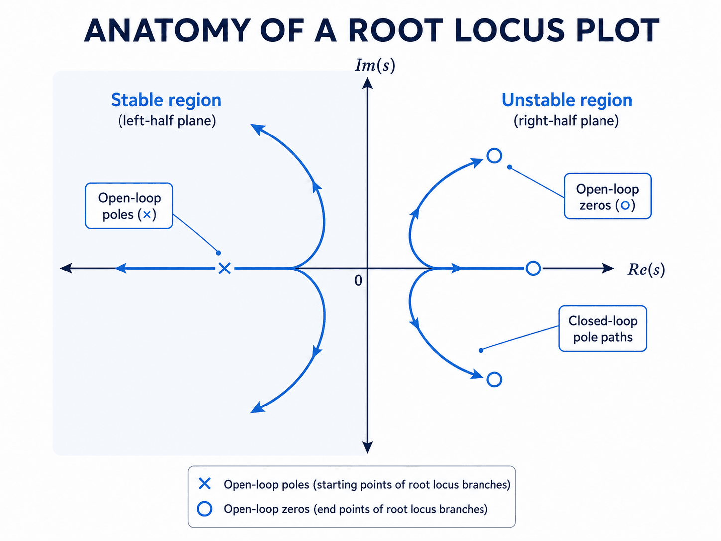
Notice that the left-half plane is the stable side for standard continuous-time linear systems. The exact closed-loop behavior depends on where the chosen gain places the poles along the locus, especially the dominant poles closest to the imaginary axis.
What Is the Root Locus Method?
The root locus method is a classical feedback control design method used to trace the roots of a closed-loop characteristic equation as a parameter changes. In most introductory and practical control design problems, that parameter is the loop gain \(K\). The method turns a polynomial stability problem into a visual design tool.
The open-loop transfer function contains poles and zeros that shape every possible closed-loop pole location. As \(K\) increases from zero toward infinity, each closed-loop pole moves along a predictable branch. If the branch crosses into the right-half plane, the closed-loop system becomes unstable. If the dominant poles sit too close to the imaginary axis, the system may be stable but slow, lightly damped, or overly oscillatory.
Root locus is especially useful in control systems engineering because it connects mathematical stability with design intuition. Instead of solving for roots at only one gain value, engineers can see the full family of possible pole locations and decide whether gain adjustment alone is enough.
The Closed-Loop Equation Behind Root Locus
Root locus starts with the closed-loop characteristic equation. For a common negative-feedback system with forward-path transfer function \(G(s)\), feedback transfer function \(H(s)\), and gain \(K\), the closed-loop pole locations are found from:
The values of \(s\) that satisfy this equation are the closed-loop poles. Root locus plots those pole locations as \(K\) varies. That is why the plot is not just a curve on a graph; it is a map of possible closed-loop dynamics.
- \(s\) Complex frequency variable. Its real part affects decay or growth, and its imaginary part affects oscillation.
- \(K\) Loop gain or adjustable parameter. Increasing \(K\) moves closed-loop poles along the locus.
- \(G(s)H(s)\) Open-loop transfer function used to identify poles, zeros, branch count, and root locus shape.
- \(\zeta\) Damping ratio used to relate dominant pole location to overshoot and oscillation.
- \(\omega_n\) Natural frequency used with damping ratio to estimate response speed and transient behavior.
Open-loop poles versus closed-loop poles
Open-loop poles and zeros come from the transfer function before closing the loop around the selected controller structure. Closed-loop poles are the roots after feedback and gain are applied. Root locus uses the open-loop pole-zero pattern to predict where the closed-loop poles can go.
Why pole location matters
For continuous-time linear systems, poles in the left-half plane generally decay over time, poles on or near the imaginary axis tend to oscillate, and poles in the right-half plane grow. The dominant poles closest to the imaginary axis usually control the visible transient response, so a design review should focus on more than simply whether every pole is technically stable.
Root Locus Rules Every Sketch Uses
Root locus construction follows a small set of rules that come from the characteristic equation. These rules help engineers sketch the plot by hand and also provide a quick way to check whether software output makes physical sense.
| Rule | What it means | Why it matters in design |
|---|---|---|
| Number of branches | The number of root locus branches equals the number of open-loop poles. | Every open-loop pole must be accounted for when reviewing the closed-loop response. |
| Starting points | Branches start at open-loop poles when \(K = 0\). | The low-gain behavior begins from the open-loop dynamics. |
| Ending points | Branches end at open-loop zeros or travel toward infinity when finite zeros are missing. | Zeros and asymptotes strongly influence where high-gain closed-loop poles move. |
| Real-axis rule | A real-axis point is on the locus if an odd number of open-loop poles and zeros lie to its right. | This identifies which real-axis segments are valid parts of the locus. |
| Symmetry | For real-coefficient systems, the root locus is symmetric about the real axis. | Complex branches and poles should appear in conjugate pairs. |
| Asymptotes | If there are more poles than zeros, excess branches go to infinity along asymptotes. | Asymptotes show where branches go when gain becomes large. |
| Angle condition | A point is on the root locus when the open-loop angle condition is satisfied. | This determines whether a candidate pole location is possible for some gain. |
| Magnitude condition | After a point is on the locus, the magnitude condition gives the gain at that point. | This connects a chosen closed-loop pole location to a practical gain value. |
How to Draw a Root Locus Plot
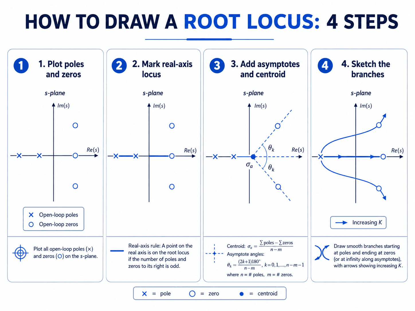
A root locus sketch is built from rules that follow the characteristic equation. Software can generate the plot quickly, but learning the hand-sketch logic helps engineers catch modeling mistakes, understand branch movement, and avoid blindly trusting a simulation.
Step 1: Plot open-loop poles and zeros
Mark each open-loop pole with an \( \times \) and each open-loop zero with an \( \circ \). The number of root locus branches equals the number of open-loop poles. Branches start at open-loop poles when \(K = 0\).
Step 2: Mark real-axis locus segments
A point on the real axis belongs to the root locus when the total number of real-axis poles and zeros to the right of that point is odd. This rule often reveals where branches begin, merge, split, or move toward zeros.
Step 3: Add asymptotes and the centroid
If the system has more open-loop poles than open-loop zeros, some branches travel toward infinity. Those branches follow asymptotes whose count equals \(n – m\), where \(n\) is the number of open-loop poles and \(m\) is the number of open-loop zeros.
The centroid \( \sigma_a \) is where the asymptotes intersect on the real axis. The asymptote angles for the standard positive-gain root locus are:
Step 4: Sketch smooth branches and direction
Final root locus branches should start at poles, end at zeros or infinity, remain symmetric about the real axis for real-coefficient systems, and follow the angle and magnitude conditions. Arrowheads show increasing \(K\), not time.
Angle Condition, Magnitude Condition, and Breakaway Points
The root locus rules are visual, but they come from two mathematical checks. The angle condition determines whether a trial point is on the locus. The magnitude condition determines the gain required to place a closed-loop pole at that point.
A point \(s\) satisfies the root locus angle condition when the total angle from the open-loop zeros minus the total angle from the open-loop poles equals an odd multiple of \(180^\circ\). Once the point is on the locus, the gain can be found from:
Breakaway and break-in points
Breakaway points occur where two or more branches leave the real axis. Break-in points occur where branches enter the real axis. A common way to find candidate points is to write \(K\) as a function of \(s\) from the characteristic equation and solve:
Not every solution is valid. Candidate breakaway or break-in points still need to lie on a valid root locus segment and match the physical branch behavior of the system.
This page assumes the standard negative-feedback convention with positive gain \(K\). If the feedback sign or gain convention changes, the locus interpretation and angle condition may change.
Worked Example: Sketching a Root Locus
A simple example shows how the rules work together. Suppose a unity-feedback system has the open-loop transfer function:
The open-loop poles are at \(s = 0\), \(s = -2\), and \(s = -4\). There are no finite open-loop zeros. Because there are three poles and zero finite zeros, the root locus has three branches and all three eventually go to infinity.
1. Branches and real-axis segments
The three branches start at \(0\), \(-2\), and \(-4\). Using the real-axis rule, the locus exists on the real-axis segment to the left of \(-4\) and on the segment between \(-2\) and \(0\). The segment between \(-4\) and \(-2\) is not on the locus because it has an even number of poles to its right.
2. Centroid and asymptote angles
Since there are three more poles than zeros, there are three asymptotes. The centroid is:
The asymptote angles are:
3. Engineering interpretation
One branch travels left along the real axis, while the other two branches leave the real axis and move into the complex plane. If those complex branches move toward or across the imaginary axis for certain gain values, the system may become lightly damped or unstable. A designer would select \(K\) only after checking the resulting closed-loop poles, transient response, and actuator requirements.
This example is intentionally simple. Real control designs often include zeros, controller dynamics, filters, delays, and higher-order poles that make software verification and engineering review essential.
How Engineers Interpret Root Locus for Design
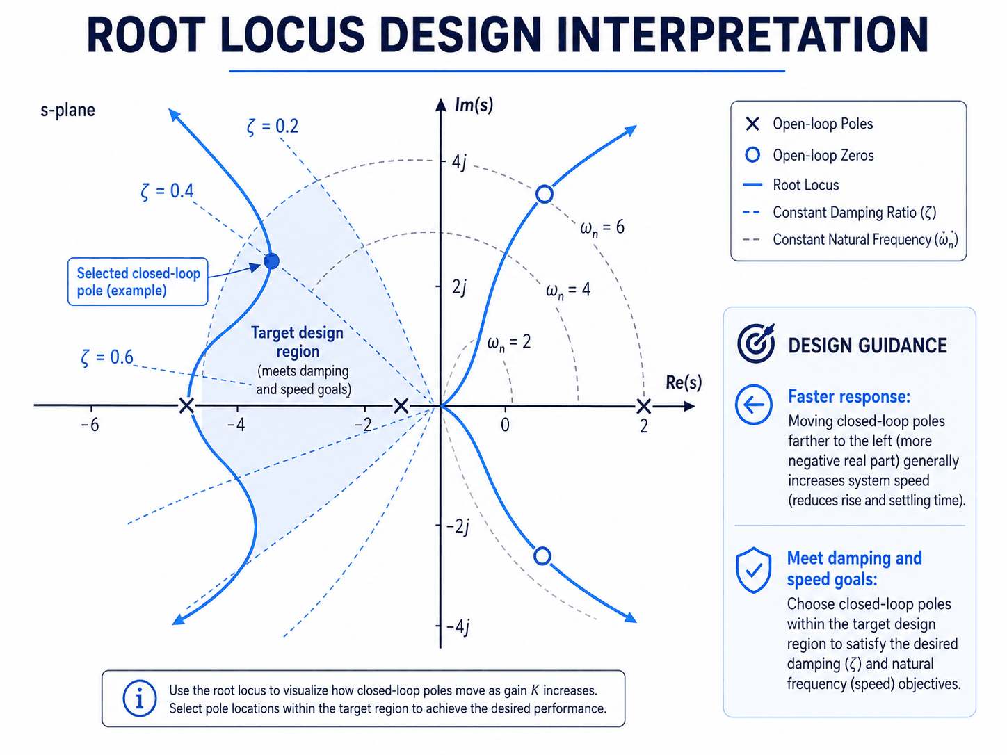
The root locus plot becomes useful when it is tied to performance requirements. A gain value is not selected because it looks convenient; it is selected because the corresponding closed-loop poles meet stability, damping, speed, and robustness goals.
Stability is the first screen, not the final answer
For a continuous-time system, closed-loop poles must stay in the left-half plane for asymptotic stability. However, a pole that is barely left of the imaginary axis may still create a response that is too slow or too oscillatory for the application.
Damping ratio and natural frequency turn the plot into a design tool
Damping ratio lines help estimate how oscillatory a dominant pole pair will be. Higher damping ratio generally moves the dominant pole direction closer to the negative real axis, while poles closer to the imaginary axis generally indicate lower damping and more oscillation. Natural frequency arcs help estimate response speed.
When a root locus branch passes through the desired design region, gain selection may be enough. When it does not, engineers usually add controller poles or zeros through lead, lag, PI, PD, or PID compensation.
When selecting a point on the locus, check all closed-loop poles for that same gain value. One selected dominant pole pair can look acceptable while another pole or lightly damped branch still causes unacceptable response.
What Controls the Shape of a Root Locus?
The shape of a root locus is controlled by the open-loop pole-zero pattern and the parameter being varied. This is why adding a controller zero, adding a controller pole, or changing a feedback structure can reshape the locus before a gain is ever selected.
| Root locus factor | Why it matters | Engineering implication |
|---|---|---|
| Open-loop pole locations | Branches start at open-loop poles when \(K = 0\). | Poles near the imaginary axis can make the uncontrolled or low-gain system slow, oscillatory, or close to instability. |
| Open-loop zero locations | Finite zeros attract branches as \(K\) becomes large. | Adding controller zeros can pull the locus toward a more desirable damping or speed region. |
| Number of poles minus zeros | This determines how many branches go to infinity along asymptotes. | High excess pole count often creates branches that are harder to keep in a desirable region with gain alone. |
| Gain \(K\) | Gain selects a point on each branch, not a new branch shape. | Gain tuning can move closed-loop poles, but it cannot fix every poor pole-zero geometry. |
| Dominant pole pair | The poles closest to the imaginary axis often dominate the transient response. | Design review should focus on the controlling poles rather than only checking that every pole is in the left-half plane. |
Root Locus Sanity Checks for Design Review
Use the following checks when reviewing a root locus plot for a control design. The goal is to catch mistakes that a clean-looking software plot can hide.
Confirm the model and feedback sign, plot poles and zeros, review branch count and real-axis segments, locate the desired pole region, select gain, then verify the closed-loop response and actuator demand before accepting the design.
| Design check | What to look for | Why it matters |
|---|---|---|
| Feedback sign | Confirm the model uses the intended negative-feedback structure. | A sign error can produce a plausible-looking plot for the wrong physical controller behavior. |
| Branch count | Count root locus branches and compare with the number of open-loop poles. | Missing a branch can hide an unstable or lightly damped closed-loop pole. |
| Real-axis rule | Check real-axis segments using the odd-number rule. | Incorrect real-axis segments lead to wrong breakaway logic and wrong gain interpretation. |
| Dominant poles | Identify which closed-loop poles are closest to the imaginary axis at the selected gain. | Dominant poles usually control overshoot, ringing, and settling behavior. |
| Response verification | Run time-response and disturbance-response checks after choosing \(K\). | Root locus predicts pole movement, but it does not automatically prove acceptable actuator effort, noise sensitivity, or robustness. |
When Gain Alone Is Not Enough
Root locus makes one limitation very visible: changing \(K\) only moves poles along the existing branches. If the locus never passes through the desired damping and speed region, a different gain will not solve the design problem. The controller structure must change.
| Design issue | What root locus shows | Typical controller response |
|---|---|---|
| Too much overshoot | Dominant branches pass through low-damping regions. | Add lead compensation or adjust controller zeros to improve damping. |
| Response too slow | Acceptable branches stay too close to the imaginary axis. | Shift dominant poles farther left if actuator and robustness limits allow. |
| Poor steady-state accuracy | Root locus may show stability but not enough low-frequency error reduction. | Use PI or lag compensation carefully, then recheck stability and transient response. |
| Branches move toward instability | Increasing gain pushes poles toward or across the imaginary axis. | Reshape the locus with controller poles and zeros rather than simply reducing performance targets. |
In practical terms, root locus is both a gain-selection tool and a controller-structure diagnostic. If the geometry is wrong, the fix is usually not “try more gain.” The fix is to change the pole-zero pattern of the loop.
Using Software to Check a Root Locus Design
Software is valuable for plotting high-order loci, selecting gain values, and checking closed-loop response. The engineering value still comes from knowing what the plot means and whether the model represents the real system well.
- Define the plant and feedback transfer function using the intended sign convention.
- Plot the root locus and compare the branch count with the number of open-loop poles.
- Overlay damping ratio and natural frequency guidance when transient response matters.
- Select a candidate gain and calculate all closed-loop poles for that gain.
- Check step response, disturbance response, control effort, and stability margins.
- Repeat with lead, lag, PI, PD, or PID compensation if the gain-only locus misses the design region.
A software root locus plot should match the expected pole count, zero count, real-axis segments, and asymptote behavior. If it does not, check the transfer function, feedback sign, units, and model simplifications before tuning the controller.
Root Locus vs Bode Plot vs Nyquist Criterion
Root locus, Bode plots, and the Nyquist criterion are all classical control tools, but they answer different questions. A strong control design often uses more than one of them.
| Method | Primary view | Best use | Common limitation |
|---|---|---|---|
| Root locus | Closed-loop pole movement as gain changes | Visual gain selection, pole-placement intuition, and compensator shaping | Less direct for frequency-domain robustness margins and noise sensitivity |
| Bode plot | Magnitude and phase versus frequency | Bandwidth, phase margin, gain margin, and frequency-response shaping | Does not directly show closed-loop pole trajectories as gain varies |
| Nyquist criterion | Complex frequency-response contour | Stability assessment for feedback loops, including challenging frequency-domain cases | Can be less intuitive for beginners and requires careful encirclement interpretation |
Root locus is often the most intuitive starting point when the main question is, “Where will the closed-loop poles go if I change gain or add a compensator?” Frequency-domain methods become especially important when bandwidth, margins, time delay, noise, and robustness drive the design.
Engineering Judgment and Field Reality
Real control systems rarely behave exactly like their clean transfer functions. Sensor noise, actuator saturation, quantization, transport delay, friction, deadband, nonlinearities, changing loads, and unmodeled dynamics can all shift the practical result away from the textbook root locus.
The method is still valuable because it gives a fast visual explanation of how feedback gain affects the poles. The engineering judgment comes from knowing when the model is good enough and when root locus needs to be supported by simulation, frequency-response review, hardware testing, or a more advanced model such as state-space analysis.
A controller that looks acceptable on root locus can still perform poorly if the actuator saturates, the sensor filters add phase lag, or the plant changes with operating condition. Always verify the selected gain against the physical system constraints.
Where the Root Locus Method Breaks Down
Root locus is built around a linear model and a varying parameter, usually scalar gain. It becomes less reliable when the actual system behavior cannot be represented well by that model or when the design objective depends on effects the plot does not show directly.
- Strong nonlinear behavior: Saturation, backlash, friction, and dead zones can change the response after the controller leaves the small-signal operating range.
- Large time delays: Delays add phase lag and may require frequency-domain or time-delay-aware analysis beyond a simple pole-zero sketch.
- Multi-input, multi-output systems: Classical root locus is most natural for SISO systems; state-space and multivariable methods may be more appropriate for coupled systems.
- Uncertain plant parameters: If mass, stiffness, resistance, load, or process gain varies widely, one root locus may not represent all important operating cases.
- Noise and actuator effort: Root locus focuses on pole location, so it does not directly reveal noise amplification, control effort, saturation risk, or implementation limits.
Common Root Locus Mistakes and Practical Checks
Most root locus errors come from confusing the visual sketch with the full design decision. A correct plot can still lead to a poor controller if the designer ignores assumptions, chooses the wrong branch, or fails to verify the final closed-loop response.
- Confusing open-loop and closed-loop poles: The plotted branches are possible closed-loop pole locations, but they are built from the open-loop pole-zero pattern.
- Assuming stable means acceptable: A stable closed-loop system can still have too much overshoot, excessive settling time, or poor disturbance rejection.
- Ignoring all poles at the selected gain: Selecting one point on the locus also fixes the other closed-loop poles for that same \(K\).
- Forgetting controller structure: Gain changes position along the existing locus; adding compensator poles and zeros changes the locus itself.
- Skipping model validation: Root locus depends on the transfer function. If the model is wrong, the plot can be mathematically clean and physically misleading.
Do not choose \(K\) only because the branch crosses into the left-half plane. Choose \(K\) because the full closed-loop system meets stability, damping, speed, control effort, and robustness requirements.
Useful Reference and Design Context
Root locus is a method from classical control theory rather than a code-based design requirement. The most useful references are technical control-system tutorials, university notes, and software documentation that connect the plot to closed-loop performance.
- University of Michigan Control Tutorials: Root Locus Controller Design tutorial explains closed-loop poles, gain selection, root locus plotting, and performance-region interpretation in a practical control design workflow.
- Project-specific criteria: Control designs should still be checked against the actual plant model, actuator limits, sensor behavior, safety requirements, and operating envelope.
- Engineering use: Use root locus as a design reasoning tool, then validate the selected controller with closed-loop response, robustness, and implementation checks.
Frequently Asked Questions
The root locus method is used to see how closed-loop pole locations change as gain or another system parameter changes. Engineers use it to judge stability, damping, response speed, oscillation tendency, and whether a proportional gain or compensator can meet performance goals.
To draw a root locus plot, identify the open-loop poles and zeros, mark the real-axis portions that satisfy the odd-number rule, calculate asymptotes and their centroid when poles exceed zeros, estimate breakaway or break-in behavior, then sketch smooth branches from poles toward zeros or infinity as gain increases.
In a root locus plot, open-loop poles are the starting points of the branches when gain is zero. Open-loop zeros are end points for branches as gain becomes very large. If there are fewer zeros than poles, the remaining branches travel toward infinity along asymptotes.
The real-axis rule says that a point on the real axis belongs to the root locus if the number of open-loop poles and zeros to the right of that point is odd. This rule helps determine which real-axis segments are part of the locus.
No. Root locus shows how closed-loop poles move in the s-plane as gain changes, while a Bode plot shows frequency response magnitude and phase versus frequency. Root locus is strongest for visual pole-placement intuition, while Bode plots are better for gain margin, phase margin, bandwidth, and frequency-domain robustness.
Summary and Next Steps
The root locus method shows how closed-loop poles move as gain changes, making it one of the clearest visual tools in classical control systems engineering. It helps connect transfer functions, stability, damping, natural frequency, and controller tuning into one s-plane design view.
The practical workflow is to understand the open-loop poles and zeros, apply root locus rules, sketch or plot the locus, identify the desired pole region, select gain or compensation, and verify the full closed-loop response. Root locus is powerful, but it should be supported by response simulation, frequency-domain review, and real system constraints.
Where to go next
Continue your learning path with related Turn2Engineering resources.
-
Stability Analysis
Learn how engineers determine whether a control system remains bounded, predictable, and safe under feedback.
-
Bode Plots
Study frequency-response methods that complement root locus with gain margin, phase margin, and bandwidth insight.
-
Feedback Control
Review the feedback concept that makes closed-loop pole movement and root locus design meaningful.