Key Takeaways
- Definition: The Navier-Stokes equation is the momentum balance for real fluids, accounting for acceleration, pressure, viscosity, and body forces.
- Main use: Engineers use it to analyze velocity and pressure fields in pipes, ducts, channels, aerodynamics, hydraulics, and computational fluid dynamics.
- Watch for: The equation is not usually solved by simple algebra; boundary conditions, flow regime, viscosity, and turbulence modeling often control the answer.
- Outcome: After reading, you should understand what each term means, when simplified forms apply, and how to sanity-check a Navier-Stokes setup.
Table of Contents
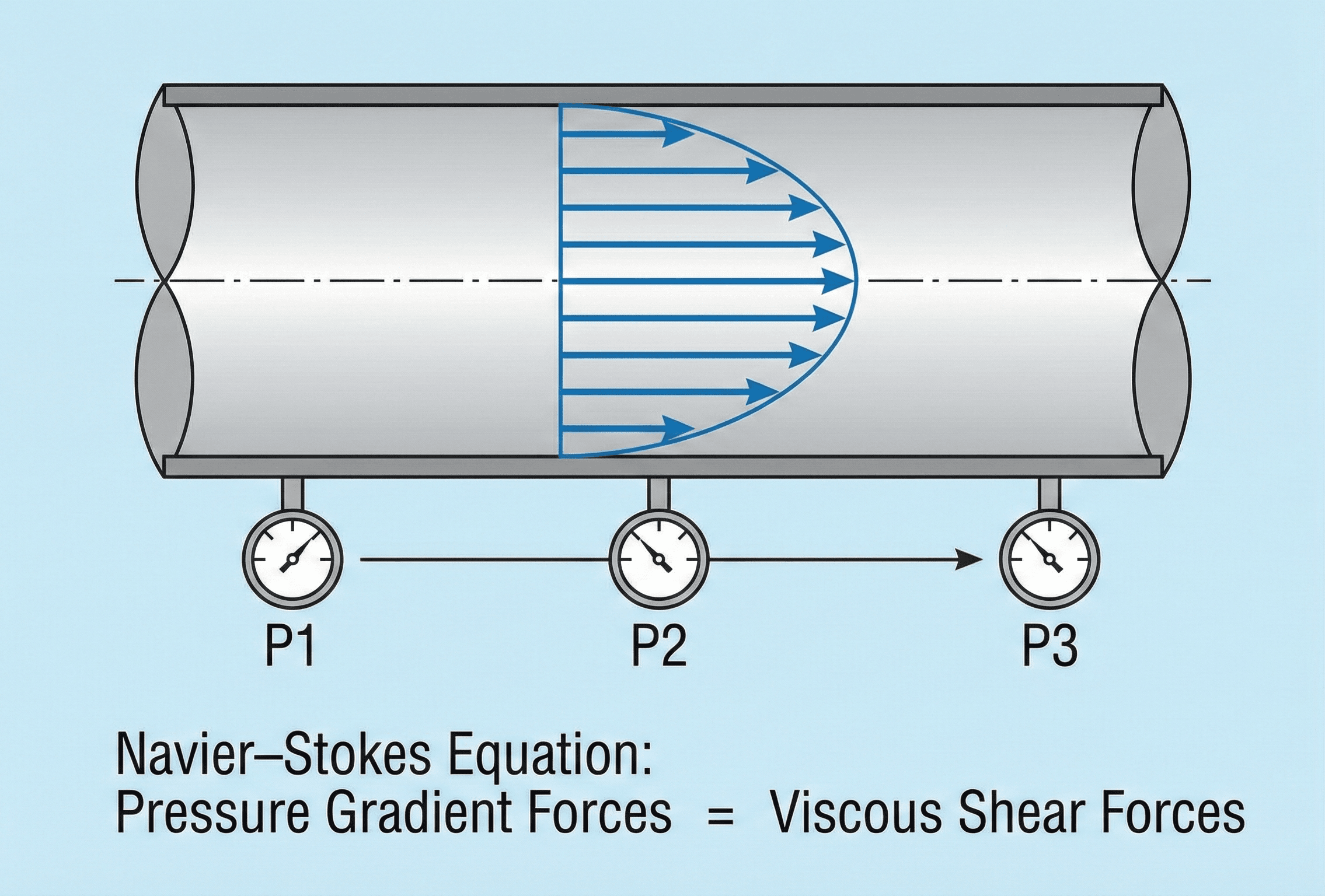
Velocity, pressure, and viscous forces in fluid motion
The Navier-Stokes equation relates fluid acceleration to pressure gradients, viscous stresses, and body forces in moving fluids.
The first thing to notice is that the equation is a force balance per unit volume, not just a pipe-flow shortcut. It tracks how a small fluid element accelerates because pressure, viscosity, and body forces are not perfectly balanced.
What is the Navier-Stokes equation?
The Navier-Stokes equation is the governing momentum equation for viscous fluid flow. In plain engineering language, it says that a fluid accelerates when pressure forces, viscous forces, gravity, or other body forces create a net imbalance.
The equation is central to fluid mechanics because it connects velocity and pressure fields rather than treating flow as a single number. That makes it the foundation behind pipe-flow analysis, aerodynamics, hydraulics, pump and turbine modeling, weather simulation, blood-flow modeling, and computational fluid dynamics.
The practical problem for most readers is usually not “Can I solve the full equation by hand?” It is more specific: which terms matter, what assumptions simplify the equation, and when should a simplified equation like the Bernoulli equation or the continuity equation be used alongside it?
The Navier-Stokes equation formula
A common vector form for an incompressible Newtonian fluid with constant density and viscosity is:
This form is often the best starting point because it clearly separates the major physical effects. The left side is fluid inertia: local acceleration plus convective acceleration. The right side contains pressure-gradient force, viscous diffusion of momentum, and body force such as gravity.
For incompressible flow, the momentum equation is paired with mass conservation:
That companion equation is not optional in most incompressible-flow problems. It says the velocity field must be divergence-free, meaning fluid volume is not locally created or destroyed.
Do not treat Navier-Stokes as one standalone algebraic formula. A usable problem also needs geometry, boundary conditions, fluid properties, initial conditions if unsteady, and a compatible continuity equation.
Variables and units in the Navier-Stokes equation
The variables in the Navier-Stokes equation represent field quantities. That means velocity and pressure vary with location, and in unsteady problems they also vary with time.
- \(\rho\) Fluid density, usually in kg/m\(^3\) or slug/ft\(^3\). Density controls the magnitude of inertial effects.
- \(\mathbf{u}\) Velocity vector field, commonly in m/s or ft/s. Components may be written as \(u\), \(v\), and \(w\).
- \(t\) Time, usually in seconds. The partial derivative with respect to time captures local unsteady acceleration.
- \(p\) Pressure field, usually in pascals or psi. The pressure-gradient term drives acceleration from high pressure toward low pressure.
- \(\mu\) Dynamic viscosity, usually in Pa·s or lb·s/ft\(^2\). Viscosity controls momentum diffusion and wall-shear effects.
- \(\mathbf{g}\) Body acceleration vector, commonly gravity in m/s\(^2\) or ft/s\(^2\).
In SI units, each term in the incompressible momentum equation has units of force per unit volume, N/m\(^3\). Checking that common unit is one of the fastest ways to catch a missing density, pressure-gradient, or viscosity term.
| Term | Physical meaning | SI unit check | Common interpretation |
|---|---|---|---|
| \(\rho \frac{\partial \mathbf{u}}{\partial t}\) | Local acceleration | N/m\(^3\) | Velocity changing with time at a fixed point |
| \(\rho(\mathbf{u}\cdot\nabla)\mathbf{u}\) | Convective acceleration | N/m\(^3\) | Velocity changing because fluid moves through a spatial velocity gradient |
| \(-\nabla p\) | Pressure-gradient force | N/m\(^3\) | Driving or resisting force caused by pressure variation |
| \(\mu\nabla^2\mathbf{u}\) | Viscous diffusion | N/m\(^3\) | Momentum transfer caused by viscosity and velocity curvature |
| \(\rho\mathbf{g}\) | Body force | N/m\(^3\) | Gravity or another force acting throughout the fluid volume |
Where the Navier-Stokes equation comes from
The Navier-Stokes equation comes from applying Newton’s Second Law to a moving fluid element or control volume. In other words, it is a momentum balance written for a material that can deform continuously instead of moving like a rigid body.
The acceleration term uses the material derivative because a fluid particle can experience two kinds of acceleration. It can speed up or slow down at a fixed point as time changes, and it can also accelerate by moving into a different part of the velocity field.
The pressure-gradient term comes from normal stresses acting on the fluid element. The viscous term comes from shear stresses generated when nearby fluid layers move at different speeds. For a Newtonian fluid with constant viscosity, those viscous stresses reduce to the compact \(\mu\nabla^2\mathbf{u}\) term in the incompressible form.
Where engineers use the Navier-Stokes equation
Engineers rarely write the full equation just to perform hand arithmetic. Instead, they use it as the governing model behind simplified equations, analytical solutions, numerical simulations, and design checks.
- Pipe and duct flow: estimating pressure drop, velocity profile, wall shear, and flow regime before using pipe-friction methods.
- Aerodynamics: modeling lift, drag, boundary layers, separation, and wake behavior around vehicles, aircraft, blades, and structures.
- Hydraulics: studying water movement in channels, outlets, spillways, valves, pumps, and pressurized systems.
- CFD analysis: solving discretized momentum and continuity equations over a computational mesh.
- Thermal-fluid systems: coupling fluid motion with heat transfer when velocity fields control convection.
Use the full Navier-Stokes framework when velocity and pressure vary spatially, viscous forces matter, boundary layers matter, or the flow cannot be captured by a one-dimensional energy equation alone.
Use a simplified equation when the assumptions are clear: continuity for mass conservation, Bernoulli for idealized mechanical energy, Darcy-Weisbach or Hazen-Williams for pipe head loss, and Reynolds number to judge the relative importance of inertia and viscosity.
Worked example: simplified flow between parallel plates
Example problem
A viscous incompressible fluid flows steadily between two large, stationary, parallel plates separated by a gap \(h\). The pressure decreases in the \(x\)-direction, and the flow is fully developed, so the velocity only varies with \(y\). Find the simplified governing equation for the velocity profile.
Start with the \(x\)-momentum form of Navier-Stokes. For steady, fully developed, one-directional flow, the acceleration terms drop out because velocity does not change with time or along the flow direction.
Rearranging shows that velocity curvature is controlled by the pressure gradient and viscosity:
If the plates are stationary, the no-slip boundary conditions are \(u(0)=0\) and \(u(h)=0\). Integrating twice gives the classic parabolic velocity profile for pressure-driven laminar flow between plates:
The maximum velocity occurs near the center of the gap, and the velocity is zero at both walls because of the no-slip condition. Higher pressure gradient increases speed, while higher viscosity resists motion.
Assumptions behind the common incompressible form
The compact form shown near the top of this page is powerful, but it is not the only version of Navier-Stokes. It relies on several assumptions that should be checked before using it as the governing equation.
- 1 The fluid is treated as a continuum, so molecular-scale effects are not controlling the flow.
- 2 Density is constant or nearly constant, making the incompressible continuity condition reasonable.
- 3 The fluid is Newtonian, meaning shear stress is proportional to rate of strain.
- 4 Dynamic viscosity is constant enough that the viscous term can be written as \(\mu\nabla^2\mathbf{u}\).
- 5 Boundary conditions such as no-slip walls, inlets, outlets, and symmetry planes are defined correctly.
Neglected or simplified factors
In real projects, the simplified incompressible form may neglect compressibility, non-Newtonian rheology, temperature-dependent viscosity, multiphase behavior, cavitation, chemical reaction, turbulence modeling details, or moving/deforming boundaries.
Do not use the constant-density incompressible form blindly for high-speed gas flow, strong heating, shock waves, slurries, foams, blood-like non-Newtonian fluids, or flows where phase change affects momentum.
Engineering judgment and field reality
The Navier-Stokes equation is exact for many continuum Newtonian-fluid assumptions, but real engineering decisions depend on how well the model represents geometry, boundary conditions, fluid properties, and flow regime.
In a real pipe, duct, valve, pump, or channel, small details can dominate the result: roughness, bends, entrance effects, partial blockage, vibration, temperature gradients, and imperfect boundary-condition data can matter more than the neat equation form.
Before trusting a detailed Navier-Stokes or CFD result, estimate the Reynolds number, check continuity, compare expected pressure drop against a simpler method, and verify that wall and inlet conditions match the actual system.
This is why experienced engineers often use the Navier-Stokes equation as the physics foundation, then validate against simpler equations, test data, field measurements, or known benchmark solutions.
Common mistakes and engineering checks
- Forgetting continuity: a velocity field that violates mass conservation is not physically valid for incompressible flow.
- Dropping terms too early: removing acceleration, viscosity, gravity, or pressure terms without checking scale can lead to the wrong model.
- Confusing pressure with pressure gradient: fluid acceleration is driven by spatial pressure change, not absolute pressure alone.
- Ignoring Reynolds number: laminar, transitional, and turbulent flows require different levels of modeling judgment.
- Using CFD as a black box: mesh quality, turbulence model, wall treatment, convergence, and boundary conditions can control the result.
If your solution predicts nonzero velocity at a stationary solid wall, violates expected symmetry, creates flow from nowhere, or gives pressure changes wildly different from a back-of-envelope estimate, stop and recheck the setup.
| Check item | What to verify | Why it matters |
|---|---|---|
| Continuity | Confirm \(\nabla\cdot\mathbf{u}=0\) for incompressible flow | Prevents nonphysical mass creation or loss |
| Boundary conditions | Check no-slip walls, inlet profiles, outlets, and symmetry assumptions | Boundary conditions often control the solution more than the equation form |
| Flow regime | Estimate Reynolds number before choosing laminar or turbulent modeling | Determines whether a simple analytical solution is realistic |
| Units | Confirm every term has units of force per unit volume | Catches missing density, viscosity, or length-scale factors |
Frequently asked questions
The Navier-Stokes equation describes conservation of momentum in a fluid. It balances fluid acceleration with pressure-gradient forces, viscous forces, body forces, and unsteady flow effects.
For an incompressible Newtonian fluid with constant density and viscosity, it is commonly written as \(\rho(\partial\mathbf{u}/\partial t+\mathbf{u}\cdot\nabla\mathbf{u})=-\nabla p+\mu\nabla^2\mathbf{u}+\rho\mathbf{g}\), paired with \(\nabla\cdot\mathbf{u}=0\).
It is difficult because velocity and pressure are coupled, the convective acceleration term is nonlinear, and turbulent flows can contain many interacting length and time scales.
Bernoulli’s equation is a simplified energy relationship often used for idealized steady inviscid flow. Navier-Stokes is the broader momentum equation that keeps acceleration, pressure, viscosity, and body-force effects.
Summary and next steps
The Navier-Stokes equation is the core momentum equation for viscous fluid flow. It explains how velocity and pressure fields develop when inertia, pressure gradients, viscosity, and body forces interact.
The most important engineering judgment is deciding which terms matter. For simple hand checks, you may use simplified forms or related equations. For complex separated, turbulent, three-dimensional, or unsteady flow, the full Navier-Stokes framework usually requires numerical methods and careful validation.
Where to go next
Continue your learning path with these curated next steps.
-
Prerequisite: Continuity Equation
Build the conservation-of-mass foundation needed for incompressible Navier-Stokes problems.
-
Current topic: Navier-Stokes Equation
Use this page as your reference for the main equation, term meanings, assumptions, and engineering checks.
-
Advanced check: Reynolds Number
Learn how engineers compare inertial and viscous effects before selecting a laminar, turbulent, or simplified flow model.