Key Takeaways
- Definition: Planck’s Law describes the spectral radiation emitted by an ideal blackbody based on wavelength or frequency and temperature.
- Main use: Engineers use it for thermal radiation, infrared sensing, pyrometry, heat-transfer estimates, optics, solar analysis, and blackbody-source calibration.
- Watch for: Real materials are not perfect blackbodies; emissivity, wavelength band, surface condition, and sensor response can dominate real measurements.
- Outcome: You will understand the formula, variables, units, blackbody assumptions, related radiation laws, and practical checks before applying the equation.
Table of Contents
Blackbody radiation intensity changes with wavelength and temperature
Planck’s Law relates blackbody spectral radiance to wavelength and absolute temperature, showing how emitted radiation shifts as temperature changes.
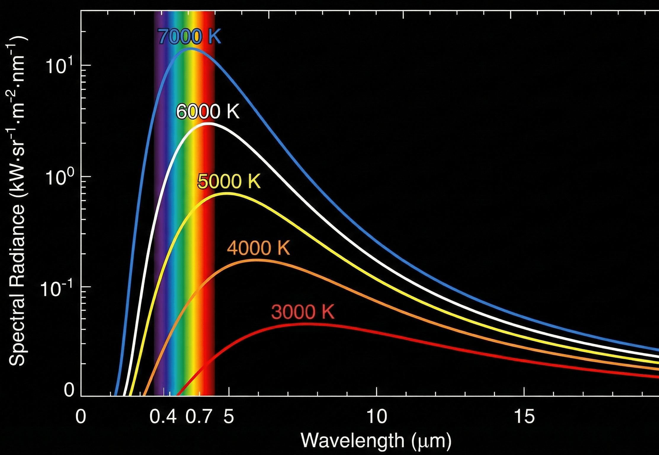
The first thing to notice is the shape of the curve. Planck’s Law is not just a total heat-radiation equation; it predicts how emitted energy is distributed across wavelength.
What is Planck’s Law?
Planck’s Law is the fundamental equation for the spectrum of thermal radiation emitted by an ideal blackbody. It tells you how much radiative energy is emitted at each wavelength or frequency for a given absolute temperature.
In engineering language, Planck’s Law connects temperature to the color, intensity, and spectral distribution of thermal radiation. It explains why a heated object first emits mostly infrared radiation, then glows red, then shifts toward shorter visible wavelengths as temperature rises.
The equation is especially important in heat transfer, thermal imaging, infrared thermometry, furnace monitoring, solar-energy analysis, radiation shields, optical sensors, and calibration sources.
The Planck’s Law formula
The most common wavelength form of Planck’s Law for blackbody spectral radiance is:
This form gives spectral radiance per unit wavelength. It shows that radiation depends strongly on wavelength \(\lambda\) and absolute temperature \(T\), with the exponential term controlling the steep drop at short wavelengths.
Planck’s Law is also written in frequency form:
The wavelength and frequency forms describe the same blackbody spectrum, but they are not interchangeable by simply substituting \(\nu=c/\lambda\). The units and differential intervals are different, so use the form that matches your data or instrument.
For a real gray or spectral surface, engineers often apply emissivity to the ideal blackbody result:
Confirm whether your problem needs spectral radiance, total radiated power, peak wavelength, or detector-band signal. Planck’s Law gives the spectrum, not automatically the total heat loss from a real surface.
Variables and units
Planck’s Law is sensitive to units because wavelength appears to the fifth power and inside an exponential. Use SI units consistently unless the equation has been explicitly converted.
- \(B_{\lambda}\) Blackbody spectral radiance per unit wavelength. Common SI unit: W/(m\(^2\)·sr·m). Often converted to W/(m\(^2\)·sr·µm) for infrared work.
- \(B_{\nu}\) Blackbody spectral radiance per unit frequency. Common SI unit: W/(m\(^2\)·sr·Hz).
- \(\lambda\) Wavelength. SI unit: meters (m). Infrared calculations often use micrometers, but the formula requires conversion unless rewritten.
- \(\nu\) Frequency. SI unit: hertz (Hz). It relates to wavelength by \(\nu=c/\lambda\) in vacuum.
- \(T\) Absolute temperature. SI unit: kelvin (K). Do not use Celsius directly inside Planck’s Law.
- \(h\) Planck constant. SI unit: J·s. It links photon energy to frequency.
- \(c\) Speed of light in vacuum. SI unit: m/s.
- \(k_B\) Boltzmann constant. SI unit: J/K. It connects temperature to thermal energy scale.
Use wavelength in meters and temperature in kelvin when using the SI form. Convert \(10\,\mu\text{m}\) to \(10\times10^{-6}\,\text{m}\), and convert \(25^\circ\text{C}\) to \(298.15\,\text{K}\).
| Symbol | Meaning | SI units | Common practical units | Engineering note |
|---|---|---|---|---|
| \(B_{\lambda}\) | Spectral radiance per wavelength | W/(m\(^2\)·sr·m) | W/(m\(^2\)·sr·µm) | Match the output unit to the wavelength interval used by the instrument. |
| \(\lambda\) | Wavelength | m | nm, µm | Small unit errors are amplified because \(\lambda^5\) appears in the denominator. |
| \(T\) | Absolute temperature | K | K after converting from °C or °F | Radiation changes very strongly with temperature. |
| \(\varepsilon_{\lambda}\) | Spectral emissivity | dimensionless | 0 to 1 | Real surfaces emit less than an ideal blackbody at the same temperature. |
Objects near room temperature emit strongly in the infrared, not the visible range. A thermal camera usually cares about a wavelength band, not a single exact wavelength.
Worked example: spectral radiance at an infrared wavelength
Example problem
Estimate the blackbody spectral radiance at \(\lambda=10\,\mu\text{m}\) for a surface at \(T=300\,\text{K}\). Use the wavelength form of Planck’s Law.
Convert the wavelength to meters:
Substitute the values into the wavelength form:
Using \(h=6.626\times10^{-34}\,\text{J·s}\), \(c=2.998\times10^8\,\text{m/s}\), and \(k_B=1.381\times10^{-23}\,\text{J/K}\), the result is approximately:
Converted to a per-micrometer interval, this is:
A 300 K object emits strongly near the thermal infrared band. This is why infrared cameras and non-contact thermometers often operate around mid- or long-wave infrared wavelengths.
Where engineers use Planck’s Law
Planck’s Law is most useful when the wavelength distribution of thermal radiation matters. Total heat-transfer equations can miss the details needed for sensors, optics, calibration, and spectral measurements.
- Infrared thermography: estimating emitted radiation in a detector wavelength band and interpreting apparent temperature.
- Pyrometry: relating spectral radiance to temperature for non-contact furnace, metal, glass, or process measurements.
- Thermal radiation heat transfer: connecting blackbody emission to real-surface emissivity and radiation exchange.
- Optical and detector design: matching source spectra, filters, detector response, and calibration curves.
- Solar and high-temperature systems: comparing emission spectra from hot surfaces, flames, lamps, or solar-like sources.
If the instrument measures a wavelength band, integrate Planck’s Law over that band and include detector response. A single-wavelength value may not represent the measured signal.
Assumptions and limitations
Planck’s Law is exact for an ideal blackbody in thermal equilibrium. Real engineering surfaces usually need additional assumptions about emissivity, viewing geometry, temperature uniformity, and detector response.
- 1 The source behaves like an ideal blackbody, or emissivity is known well enough to correct the blackbody result.
- 2 The surface temperature is uniform or the calculation clearly represents an effective radiating temperature.
- 3 Wavelength, temperature, and constants are used in a consistent unit system.
- 4 Reflections, atmosphere, optics, window transmission, and detector spectral response are either negligible or handled separately.
Neglected factors
The simple blackbody form does not include spectral emissivity, surface roughness, oxidation, reflected background radiation, atmospheric absorption, view factor, finite sensor bandwidth, or nonuniform temperature across the target.
Do not use a perfect-blackbody calculation as a final temperature measurement for shiny metals, glass through windows, flames, partially transparent gases, or surfaces with unknown emissivity.
Using Planck’s Law in software
Engineers often implement Planck’s Law in spreadsheets, Python, MATLAB, or sensor-processing scripts. The two biggest practical issues are unit consistency and numerical stability in the exponential term.
- Excel: Convert wavelength to meters and temperature to kelvin before using the exponential term. Keep constants in separate cells to avoid hidden unit mistakes.
- Python: Use NumPy arrays for wavelength sweeps and plot \(B_{\lambda}\) versus \(\lambda\) for different temperatures.
- MATLAB / scripts: Use vectorized wavelength arrays and convert output to W/(m\(^2\)·sr·µm) when matching infrared-instrument data sheets.
If a plotted Planck curve is off by orders of magnitude, check wavelength units first. Mixing micrometers and meters is the most common implementation mistake.
Engineering judgment and field reality
In real thermal-radiation work, the hard part is rarely typing Planck’s Law. The hard part is knowing what the sensor actually sees and whether the target behaves enough like a blackbody.
A thermal camera pointed at polished metal may report a misleading temperature because the surface reflects surrounding radiation and has low emissivity. The Planck curve may be correct, but the measurement setup is not equivalent to a blackbody.
For temperature measurement, emissivity and background reflection can matter as much as the equation. Use known-emissivity tape, coatings, calibration targets, or contact measurements when accuracy matters.
Common mistakes and engineering checks
- Using Celsius in the exponential: Planck’s Law requires absolute temperature in kelvin.
- Mixing meters and micrometers: wavelength appears as \(\lambda^5\), so unit mistakes create enormous errors.
- Confusing spectral and total radiation: \(B_{\lambda}\) is spectral radiance, not total emitted power.
- Ignoring emissivity: real surfaces rarely emit as perfect blackbodies across all wavelengths.
- Comparing wavelength and frequency forms incorrectly: \(B_{\lambda}\) and \(B_{\nu}\) use different per-interval units.
As temperature increases, the Planck curve should rise and its peak should move toward shorter wavelengths. If your curve moves the other way, check units and constants.
| Check item | What to verify | Why it matters |
|---|---|---|
| Temperature | Use kelvin, not Celsius or Fahrenheit | The exponential term depends on absolute temperature |
| Wavelength | Convert µm or nm to meters for the SI equation | \(\lambda^5\) amplifies unit errors |
| Output basis | Confirm whether output is per meter, per micrometer, or per hertz | Spectral radiance depends on the interval definition |
| Surface behavior | Check emissivity, reflections, and transparency | Real surfaces are not always blackbodies |
Frequently asked questions
Planck’s Law describes the spectral radiance emitted by an ideal blackbody as a function of wavelength or frequency and absolute temperature.
In wavelength form, \(B_{\lambda}\) is commonly expressed in W/(m\(^2\)·sr·m) or converted to W/(m\(^2\)·sr·µm). Wavelength should be converted to meters and temperature to kelvin when using the SI equation.
Planck’s Law gives the full blackbody spectrum. Wien’s displacement law gives only the wavelength where that spectrum reaches its peak.
Real surfaces may deviate from ideal blackbody behavior because emissivity depends on wavelength, direction, temperature, oxidation, roughness, coating, and surface material.
Summary and next steps
Planck’s Law is the core equation for blackbody spectral radiation. It predicts how radiance varies with wavelength or frequency and absolute temperature, making it essential for thermal radiation, infrared sensing, and optical engineering.
The most important engineering judgment is knowing whether an ideal blackbody model is appropriate. For real surfaces, account for emissivity, wavelength band, reflections, atmospheric transmission, sensor response, and temperature uniformity before trusting the result.
Where to go next
Continue your learning path with these curated next steps.
-
Prerequisite: Heat Transfer
Build the broader foundation behind conduction, convection, radiation, and thermal-energy movement.
-
Current topic: Planck’s Law
Use this page as your reference for blackbody spectral radiance, units, constants, assumptions, and engineering checks.
-
Advanced: Planck’s Law Calculator
Apply the equation directly to compute spectral radiance or estimate temperature from measured blackbody-like radiation.