Transportation Modeling

What is transportation modeling?

Transportation modeling is the use of mathematical and computational representations of travel demand and transportation networks to predict how people and goods move under different conditions, so engineers can test scenarios and support planning, design, and operations decisions before they are built.

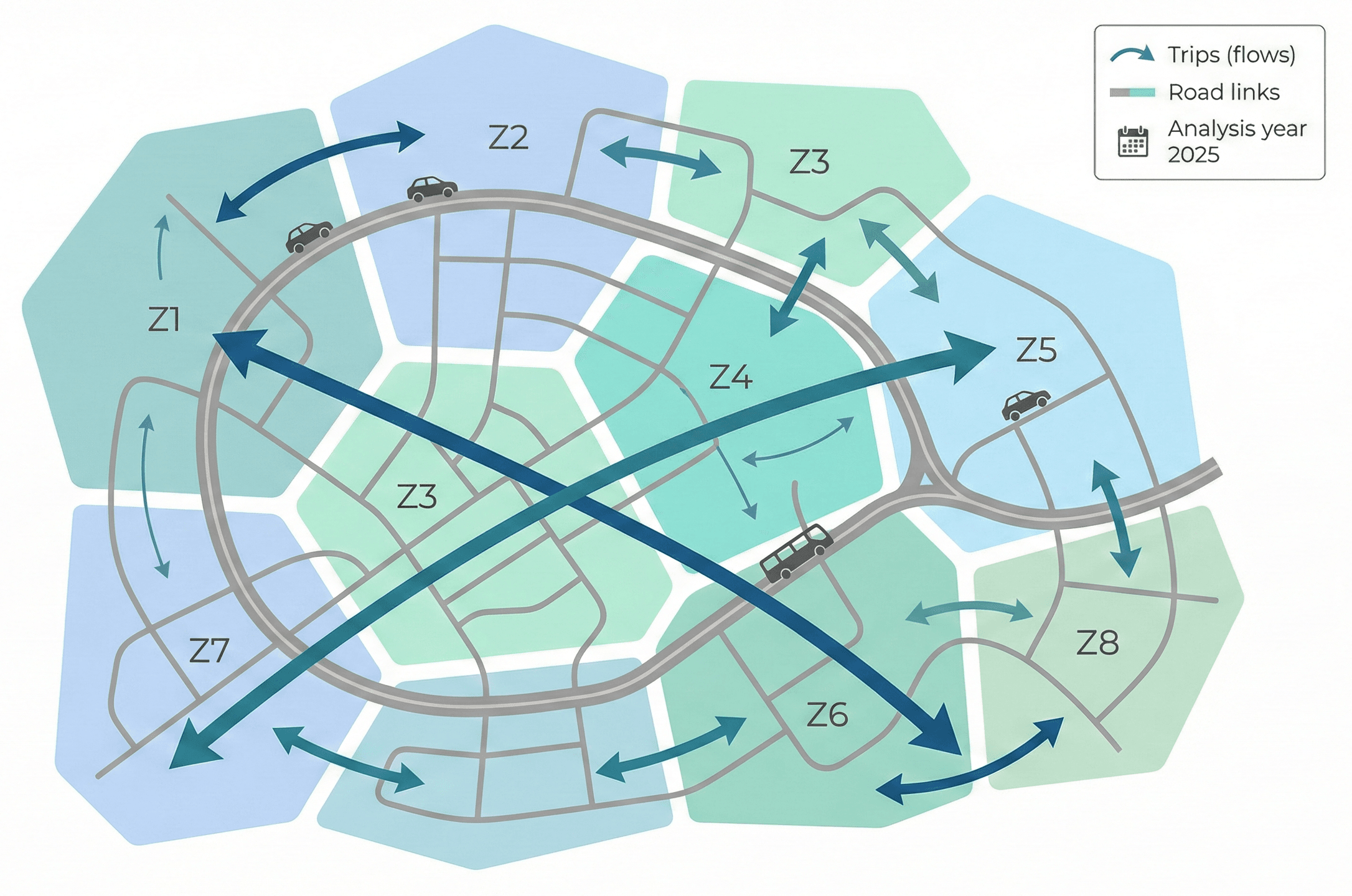
In practice, a transportation model combines two main ingredients: demand (who is traveling, from where to where, at what times, and by which modes) and supply (the road, transit, walking, cycling, and freight networks with their capacities and operating characteristics). The model then estimates how demand interacts with supply to produce volumes, speeds, delays, and other performance measures.

These models sit at the heart of many Transportation Engineering tasks, including corridor studies, long-range regional plans, highway and intersection design, transit network planning, and even policy analysis for pricing or emissions. For deeper background on the underlying traffic relationships, you can also see Turn2Engineering’s dedicated guide on Traffic Flow Theory.

Types of transportation models

Not all transportation models are built the same way. The “right” model depends on the questions being asked, the geographic scale, available data, and computing resources. At a high level, models can be categorized by spatial scale, behavioral detail, and purpose.

By spatial and temporal scale

• Macroscopic models: Treat flows like fluids, using aggregated relationships between volume, speed, and density. Regional travel demand models and many highway assignment models fall into this category.
• Mesoscopic models: Combine aggregate flow relationships with some individual-vehicle logic. They are often used when detail is needed on specific corridors but full microsimulation is too heavy.
• Microscopic models: Represent individual vehicles or travelers with car-following and lane-changing logic. Microsimulation is commonly used for detailed intersection, interchange, and corridor operations studies.

By purpose and questions

• Planning models: Answer long-term questions about land use, network expansion, and multimodal investment tradeoffs, often using the four-step travel demand framework described below.
• Operations models: Focus on short-term performance such as queue lengths, delay, and level of service (LOS) at specific facilities, often using traffic microsimulation combined with Highway Design and Highway Capacity Manual methods.
• Policy models: Explore pricing, parking, transit fare structures, or demand management, frequently relying on behavioral models like discrete choice or activity-based modeling.

The four-step travel demand modeling process

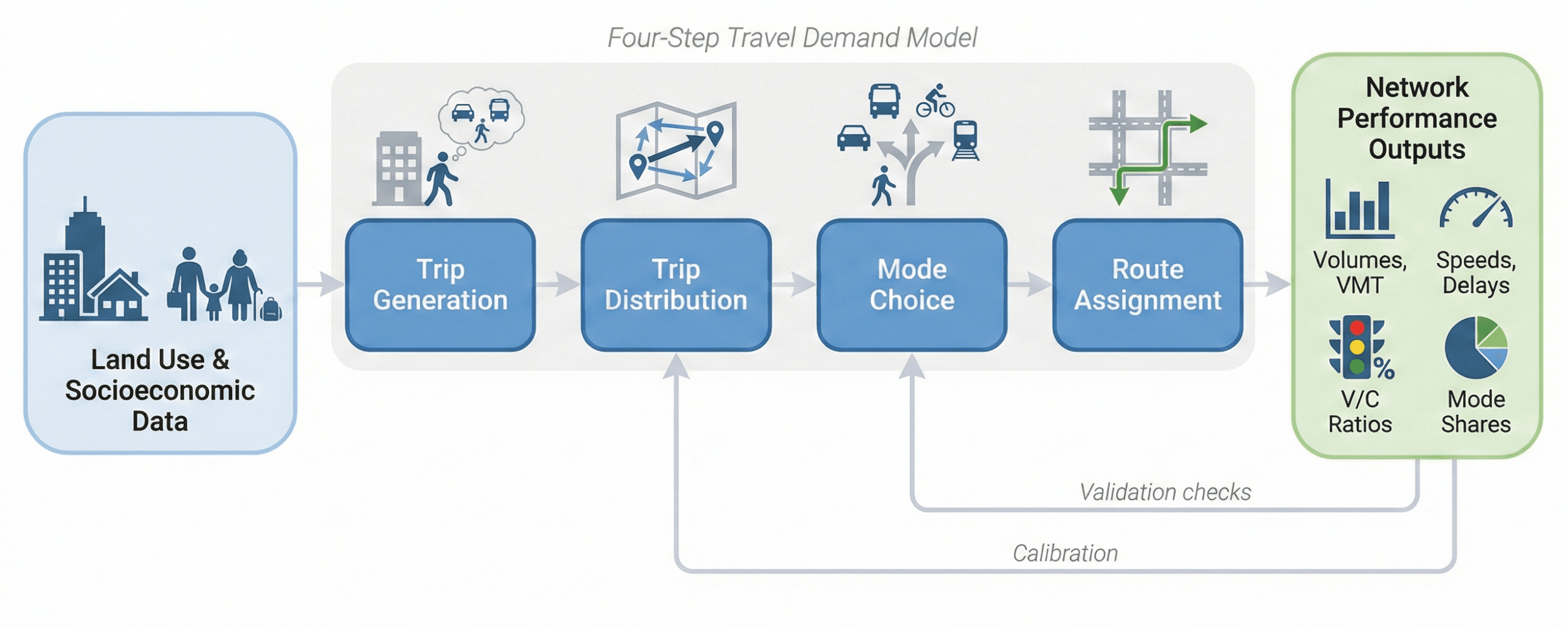
Many planning agencies still rely on the classic four-step travel demand model. While modern methods are moving toward activity-based and agent-based models, the four steps remain a useful mental model and are still widely used in practice.

1. Trip generation

Trip generation estimates how many trips originate and end in each traffic analysis zone (TAZ) for a given time period (e.g., daily or peak hour). Equations relate land use and socio-economic variables—such as households, jobs by type, income, or car ownership—to trip productions and attractions.

2. Trip distribution

Trip distribution connects productions and attractions into an origin–destination (O–D) pattern. Gravity models are common, where trips between zones decrease with increasing travel time or cost, analogous to gravitational attraction weakening with distance. The output is an O–D matrix of trips by purpose.

3. Mode choice

Mode choice splits trips among competing modes such as driving alone, carpool, bus, rail, biking, or walking. Behavioral models (often discrete choice models) relate the attractiveness of each mode to travel time, cost, reliability, comfort, and sometimes socio-economic traits of travelers.

4. Route assignment

Route (or traffic) assignment loads trips from the O–D matrix onto specific paths through the network, respecting capacity and travel time. Deterministic or stochastic user equilibrium algorithms are often used so that no traveler can reduce their travel time by unilaterally changing routes.

Key equations and performance measures

Under the hood, transportation models use many equations. One of the most important families is discrete choice models, often used for mode choice or route choice. A common form is the multinomial logit model, which converts generalized costs or utilities into mode probabilities.

Here, \(P_i\) is the probability of choosing mode \(i\), \(C_i\) is the generalized cost of mode \(i\) (combining time, money, and sometimes reliability or comfort), and \(\theta\) is a sensitivity parameter that controls how strongly travelers respond to differences in cost. Lower-cost modes receive higher probability, but all modes retain some chance of being chosen.

Common performance measures

Once trips are assigned to the network, engineers typically report:

• Link and turning volumes (vehicles/hour or passengers/hour).
• Volume-to-capacity (v/c) ratios as indicators of congestion.
• Travel times and delays by route, corridor, or origin–destination pair.
• Vehicle-miles traveled (VMT) and vehicle-hours traveled (VHT) by scenario.
• Mode shares and ridership for transit alternatives.

For detailed capacity and LOS calculations on specific facilities, a model is often paired with methods grounded in Traffic Flow Theory and Highway Capacity Manual procedures, and sometimes with interactive tools you can find in Turn2Engineering’s engineering calculators library.

Data, calibration, and validation

A transportation model is only as good as the data and calibration behind it. Even an elegant mathematical structure will mislead decision-makers if it does not replicate current conditions within acceptable error ranges.

Key data sources

• Traffic counts and screenlines: Permanent counters, short-duration tube counts, and turning-movement counts at key intersections.
• Transit boarding data: Automatic passenger counters, farebox data, or surveys that show ridership by route and stop.
• Household and workplace data: Census, surveys, or mobile device data that describe where people live, work, and travel.
• Travel time and speed data: Probe data from GPS, floating car runs, or third-party providers to validate travel times on major routes.

Calibration

Calibration adjusts model parameters—such as trip rates, friction factors in gravity models, mode choice coefficients, or capacity and speed functions—until the model reproduces observed base-year data. Engineers target metrics like link volume errors, screenline matches, and mode share differences within agreed tolerances.

Validation and reasonableness checks

After calibration, validation tests how the model behaves under slightly different conditions or against data not used in calibration. Reasonableness checks ensure that elasticities, responses to travel time or cost, and shifts between modes or routes all “look right” to experienced modelers, even before focusing on exact numerical fit.

Using transportation models in practice

In real projects, transportation models are decision-support tools. They do not “approve” projects or substitute for judgment, but they provide a structured way to compare alternatives and communicate tradeoffs to stakeholders, agencies, and the public.

Typical applications

• Corridor and highway studies: Estimate future volumes, v/c ratios, and travel times under different lane configurations, interchange designs, or managed lane strategies.
• Transit planning: Evaluate new routes, frequency changes, bus rapid transit (BRT), or rail lines by predicting ridership, mode shifts, and network-wide effects.
• Land-use and development review: Assess how new residential, commercial, or industrial developments will affect surrounding network performance and multimodal accessibility.
• Policy analysis: Explore congestion pricing, parking policy, TDM programs, or tolling strategies before implementation.

Common pitfalls and engineering checks

• Interpreting model outputs as precise forecasts rather than approximate indicators of direction and magnitude.
• Comparing scenarios with inconsistent assumptions (e.g., different land-use baselines).
• Ignoring network bottlenecks or operational details that the model does not represent explicitly.
• Presenting detailed numbers without clearly stating uncertainty and limitations.

For more conceptual background on how modeling results feed into project prioritization and policy decisions, it is helpful to pair this page with Turn2Engineering’s guide on Transportation Planning, which zooms out to the broader planning process.