Key Takeaways
- Definition: Sieve analysis determines the grain size distribution of a soil by separating particles through standard sieves and measuring the retained mass on each one.
- Use case: Engineers use it to classify soils, screen materials for fill or backfill, compare drainage behavior, and support compaction, filter, and earthwork decisions.
- Main decision: The biggest question is not just “what percent passes,” but whether the gradation actually fits the intended function, specification, and field condition.
- Outcome: After reading, you should know how to read a gradation curve, what the results mean in practice, and where sieve analysis stops being enough by itself.
Table of Contents
Introduction
In brief: Sieve analysis measures soil gradation by sorting particles through standard sieves, helping engineers classify material and judge whether it will drain, compact, or perform as intended.
Who it’s for: Students, lab staff, and geotechnical designers.
Sieve analysis is one of the first tests that turns a bag of soil into engineering information. It looks simple, but the gradation it reveals affects classification, constructability, drainage, and quality control.
Sieve Analysis infographic
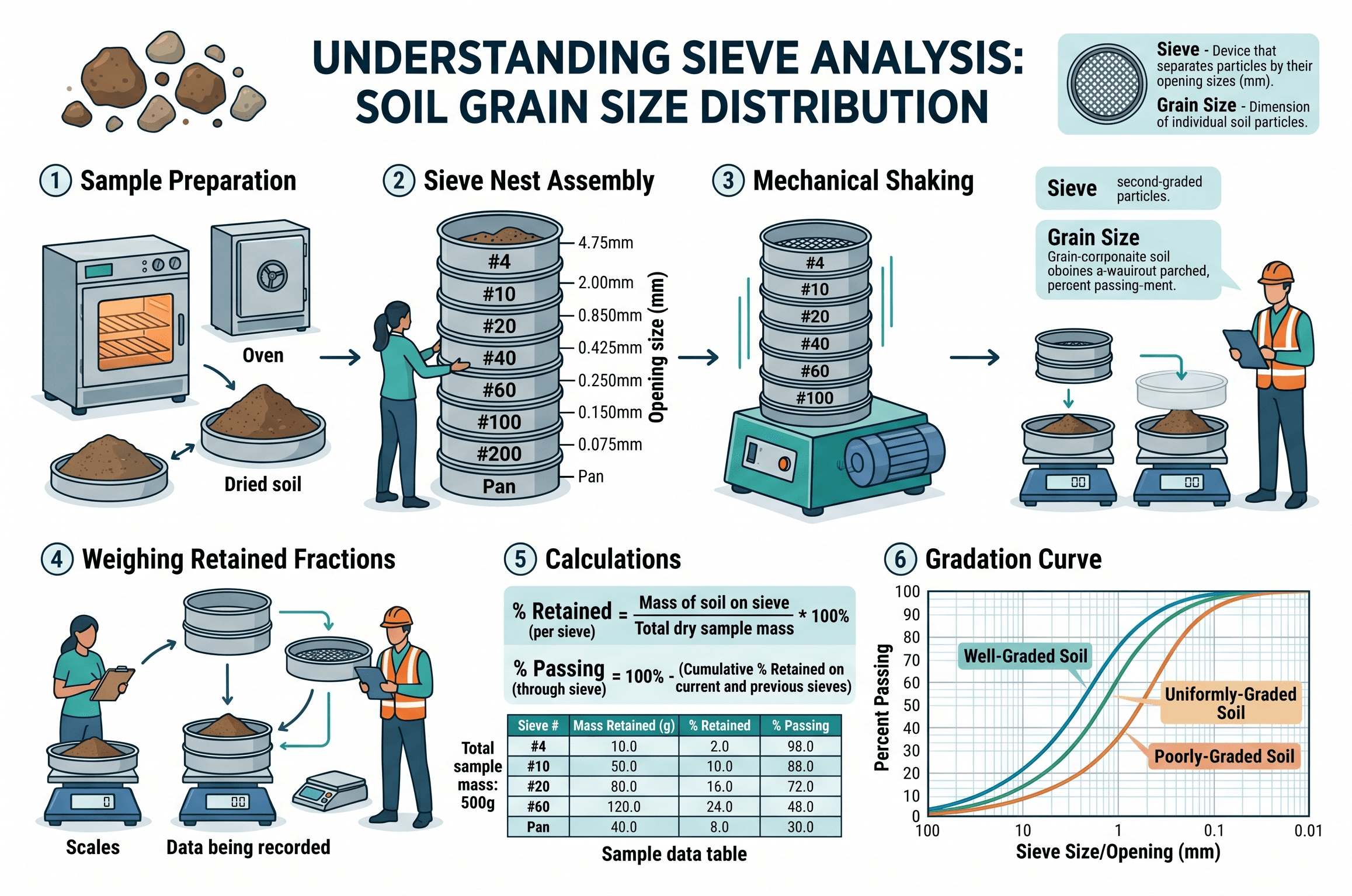
Notice the link between the physical lab setup and the final plot. The test is not just about weighing soil on sieves; it is about turning that distribution into decisions about classification, drainage, compaction, and suitability for the job.
What is Sieve Analysis?
Sieve analysis is a laboratory method used to determine the particle-size distribution of a soil by passing it through a nested stack of standard sieves and measuring how much material is retained on each sieve. The output is usually reported as percent retained, cumulative percent retained, and percent passing.
In geotechnical engineering, that information does far more than describe whether a soil is “coarse” or “fine.” Gradation affects how densely a soil can pack, how quickly water can move through it, how well it works as engineered fill, whether it may segregate during placement, and whether it is even appropriate for a particular backfill or filter application.
Sieve analysis is therefore both a classification test and a decision-support test. It helps place a material within the bigger geotechnical workflow that also includes Soil Mechanics, plasticity testing, moisture-density testing, and broader Geotechnical Data Analysis.
What the test actually tells you
The primary output of sieve analysis is gradation, meaning how particle sizes are distributed across the sample. A uniformly graded soil has most of its particles within a narrow size range. A well-graded soil spreads particles across a wider range of sizes. A gap-graded soil is missing one or more intermediate size bands.
Why gradation matters
Gradation shapes engineering behavior. Coarse, open-graded materials tend to drain quickly but may be difficult to compact into a dense, tightly interlocked structure unless the gradation and angularity are favorable. Well-graded soils often compact more efficiently because smaller grains fill the voids between larger ones. Excess fines may improve fill density in some cases but can also reduce permeability, increase frost susceptibility concerns, or change field moisture sensitivity.
Key variables and typical units
Most sieve analysis reports use mass percentages and nominal sieve sizes. The curve is usually plotted with particle size on a logarithmic horizontal axis and percent passing on a linear vertical axis.
- \(W_t\) Total dry mass of the test specimen, usually in grams.
- \(W_r\) Mass retained on a given sieve, usually in grams.
- \(\%\text{Retained}\) Percentage of total sample mass retained on a sieve.
- \(\%\text{Passing}\) Percentage of sample finer than a given sieve size.
- \(D_{10}, D_{30}, D_{60}\) Particle sizes at 10%, 30%, and 60% passing, often used to describe gradation and calculate coefficients.
- \(C_u\) Coefficient of uniformity, \(D_{60}/D_{10}\), used to indicate spread of particle sizes.
- \(C_c\) Coefficient of curvature, \(D_{30}^2/(D_{10}D_{60})\), used with \(C_u\) when discussing gradation shape.
Never judge a soil only by one passing percentage. The overall curve shape often matters more than any single sieve result when you are thinking about constructability or drainage behavior.
How engineers use sieve analysis in practice
In the real world, sieve analysis is rarely the last step. It is usually an early sorting tool that tells the engineer what deeper questions to ask next.
Start with the gradation result. If the soil is mostly coarse with low fines, think first about drainage, segregation, and whether the material can meet backfill or filter intent. If fines are meaningful, pair the result with plasticity and moisture-sensitive behavior. If the soil is intended for compaction control, connect the gradation to a Standard Proctor Test or broader Compaction Test workflow before writing field expectations.
This is why sieve analysis appears across so many project types. A gradation curve can influence subgrade evaluation, select fill approval, filter compatibility, trench backfill selection, pavement layer control, and earthwork specifications. It is also a common link between site characterization and design decisions in Geotechnical Earthworks or Ground Improvement screening.
Equations and calculations
The math behind sieve analysis is straightforward, but the interpretation is where the engineering value sits. Each retained mass is converted to a percentage of the total sample, and the cumulative retained mass is used to find percent passing.
Once the curve is plotted, engineers may estimate characteristic particle sizes such as \(D_{10}\), \(D_{30}\), and \(D_{60}\), then calculate:
These parameters help describe whether a soil appears well graded or more uniform, but they are only part of the picture. They do not replace visual observation, fines characterization, or project-specific requirements.
Worked example
Example soil sample
Suppose a dry soil specimen has a total mass of 500 g. After shaking through a sieve stack, the lab records the following retained masses:
| Sieve | Opening | Mass retained (g) | % retained | % passing |
|---|---|---|---|---|
| No. 4 | 4.75 mm | 25 | 5 | 95 |
| No. 10 | 2.00 mm | 90 | 18 | 77 |
| No. 40 | 0.425 mm | 180 | 36 | 41 |
| No. 200 | 0.075 mm | 130 | 26 | 15 |
| Pan | Finer than No. 200 | 75 | 15 | 0 |
The first takeaway is that the soil contains a meaningful coarse fraction but also 15% material finer than the No. 200 sieve. That means sieve analysis alone is not enough if classification or behavior of the fines matters. You would likely want plasticity information, and in some cases a hydrometer-based extension for the finer fraction.
The second takeaway is practical. A soil like this may still compact well, but field moisture sensitivity and drainage behavior can differ greatly from what someone might assume if they only looked at the coarse fraction. That is why gradation curves are best read as part of a broader material story, not as a stand-alone label.
Engineering judgment and field reality
Experienced engineers know that sieve analysis results can be technically correct and still mislead a project team if the sample is not representative or the material changes across the site. Borrow sources vary. Fill stockpiles segregate. Moist material can form clods that distort the apparent coarse fraction if preparation is poor. Crushed aggregate and natural soils can produce very different field behavior even when broad passing percentages look similar.
Another field reality is that contractors and inspectors often think in terms of specification bands, not gradation shape. A soil may “pass spec” and still behave poorly if it is highly gap graded, moisture sensitive, or contaminated with unexpected fines. The lab report should support judgment, not replace it.
A gradation curve from one bagged sample should never be treated as a complete site truth. In earthwork, variability across lifts, stockpiles, and borrow zones can matter as much as the reported curve itself.
When this method breaks down
Sieve analysis breaks down when the engineering problem is controlled by what happens below the No. 200 sieve, by plasticity, by soil structure, or by state-dependent behavior in the field. It tells you particle-size distribution, but it does not tell you directly whether a silt is nonplastic or highly active, whether a clay will swell, whether a compacted fill will soften under wetting, or whether a soil skeleton will collapse under load.
It is also limited when particle breakage is possible during preparation or when the sample includes cemented lumps, fragile particles, fibrous organics, or materials whose behavior is governed more by shape and surface chemistry than by nominal size. In those cases, gradation remains useful, but only as one piece of a much larger characterization effort.
For fine-grained fractions, sedimentation methods and plasticity tests often become necessary. For design applications involving seepage, settlement, or strength, you usually need to connect sieve analysis to permeability, consolidation, or shear behavior rather than stopping at the curve.
Common pitfalls and senior engineer checks
- Using a gradation result from a nonrepresentative sample and assuming it covers the whole site or stockpile.
- Ignoring the fines fraction because the material “looks sandy” in the field.
- Reading a curve without checking whether the sample was washed, dried, or prepared consistently.
- Assuming a well-graded curve automatically means good performance under all moisture conditions.
- Comparing materials on passing percentages alone without checking plasticity, angularity, or project function.
One of the most expensive mistakes is approving material for drainage or free-draining backfill based only on coarse appearance while overlooking enough fines to change permeability and clogging behavior.
Ask three questions before moving on: Is the sample representative? Does the gradation match the actual project function? What additional test would most likely change the decision if the gradation alone turned out to be misleading?
| Question | What to look for | Why it matters |
|---|---|---|
| Too much fines? | Percent passing No. 200 and whether fines appear plastic or nonplastic | Controls drainage tendency, compaction response, and classification path |
| Curve shape reasonable? | Well graded, uniform, or gap graded pattern | Affects packing, segregation, and suitability for fill or filter use |
| Need follow-up testing? | Hydrometer, Atterberg Limits, compaction, permeability, or strength testing | Prevents overconfidence from a gradation-only interpretation |
| Spec match or function match? | Not just passing the limits, but fitting the actual role of the material | Good projects care about performance, not box-checking alone |
Relevant standards and design references
Sieve analysis should be tied to the standard that matches the soil type, the project specification, and whether the fine fraction needs to be handled separately.
- ASTM D6913/D6913M: Standard sieve analysis procedure for determining the particle-size distribution of soils between 75 mm and the No. 200 sieve. This is the core reference for the sieve portion of the workflow.
- ASTM D1140: Covers determination of material finer than the No. 200 sieve by washing. This matters when accurate fine-fraction separation is needed before dry sieving.
- ASTM D7928: Extends gradation into the fine-grained fraction using sedimentation hydrometer analysis for material finer than the No. 200 sieve.
- AASHTO T 88: Widely used transportation-oriented method for particle-size analysis of soils, especially where agency specifications or DOT workflows govern.
In practice, the right reference is often set by the client, DOT, owner specification, or laboratory accreditation requirements. Always confirm the governing test method before comparing results across projects.
Frequently asked questions
Sieve analysis measures the coarse fraction by physically separating particles through standard sieves, while hydrometer analysis estimates the distribution of finer particles by how they settle in suspension. In geotechnical work, they are often paired so the final gradation covers both coarse and fine portions of the soil.
It matters because grain-size distribution strongly influences classification, drainage tendency, compaction behavior, and the direction of follow-up testing. Sieve analysis is often the first filter that tells an engineer how the material should be understood before strength, compressibility, or permeability are evaluated.
Yes. A material can fit specification bands and still underperform if the fines are problematic, the stockpile is variable, the soil is moisture sensitive, or the gradation is acceptable on paper but mismatched to the actual field function. Passing a gradation band is not the same as proving field performance.
It commonly appears in site characterization, borrow source evaluation, trench backfill selection, pavement and subgrade materials work, embankment fill approval, drainage layer design, and filter-related checks. It is one of the most common gateway tests in geotechnical laboratory programs.
Summary and next steps
Sieve analysis is simple in procedure but powerful in consequence. It gives engineers a direct look at soil gradation, and that gradation influences classification, constructability, drainage, and the way a material fits into design or quality control decisions.
The biggest practical lesson is that sieve analysis is best used as a starting point, not a final verdict. The strongest interpretations connect the curve to the material’s job on the project, then add the follow-up tests needed to reduce uncertainty where gradation alone cannot answer the real engineering question.
If you treat sieve analysis as both a measurement tool and a decision trigger, it becomes much more valuable. It helps you know what the soil is, what it might do, and what you need to test next before design assumptions harden into project risk.
Where to go next
Continue your learning path with these closely related geotechnical topics.
-
Read a deeper dive on Soil Mechanics
Build the broader intuition behind how gradation connects to stress transfer, seepage, compressibility, and shear behavior.
-
Study the Standard Proctor Test next
Useful when the next question is how gradation and water content translate into compaction performance and field targets.
-
Explore Geotechnical Data Analysis
See how lab results like gradation become part of a defensible subsurface model and material recommendation.