Key Takeaways
- Definition: Bernoulli’s Equation is a mechanical energy balance that relates pressure, velocity, and elevation along a streamline.
- Main use: Engineers use it to estimate pressure changes, flow speed, elevation effects, and idealized energy conversion in fluid systems.
- Watch for: The basic equation assumes steady, incompressible, inviscid flow and does not include pump head, turbine head, or friction losses.
- Outcome: You will be able to apply the formula, interpret each head term, rearrange it, and recognize when a more complete model is needed.
Table of Contents
Pressure, Velocity, and Elevation Head in Bernoulli’s Equation
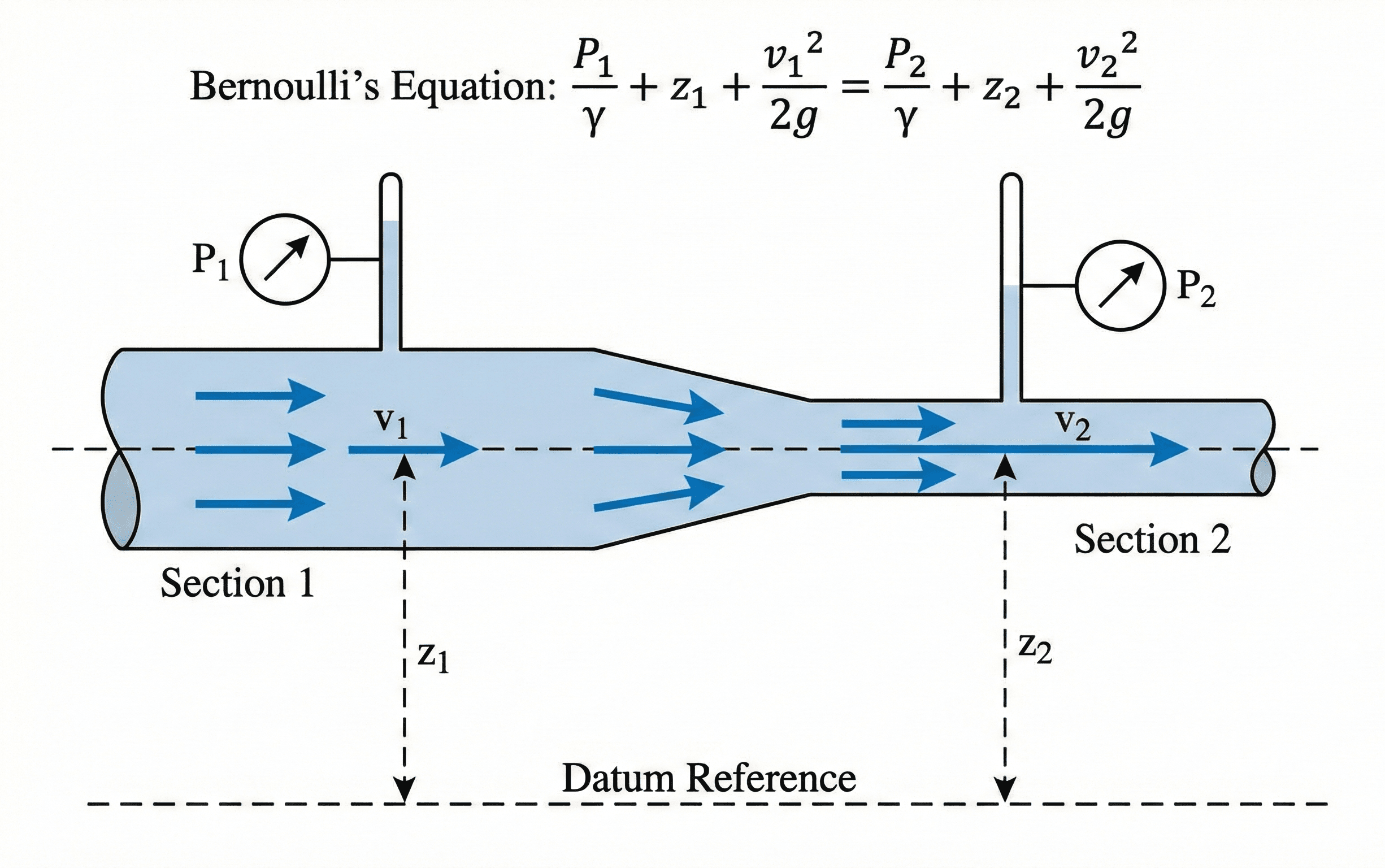
Bernoulli’s Equation relates pressure, velocity, and elevation along a streamline to show how mechanical energy shifts through flowing fluid.
Notice that none of the three energy terms must stay constant by itself. Pressure can decrease while velocity increases, elevation can consume available head, and the total idealized mechanical energy stays constant only when the assumptions are reasonable.
What is Bernoulli’s Equation?
Bernoulli’s Equation is a conservation of mechanical energy relationship for fluid flow. In its most common engineering form, it says that pressure head, velocity head, and elevation head remain constant along a streamline when the flow is steady, incompressible, and frictionless.
In practical terms, the equation helps answer questions such as: How much pressure is lost when water speeds up through a nozzle? How much velocity is created when a tank drains through an outlet? How much static pressure is available at a lower elevation? These are common fluid mechanics questions in pipes, nozzles, tanks, venturi meters, irrigation layouts, pump suction checks, and introductory hydraulics.
The important engineering idea is not just the algebra. Bernoulli’s Equation teaches that pressure, speed, and height are different forms of the same idealized mechanical energy. When one rises, another often falls.
The Bernoulli’s Equation formula
The head form is the most useful starting point for many civil, mechanical, and environmental engineering problems because every term has units of length. That makes it easier to compare pressure, velocity, and elevation on the same scale.
Between two points on the same streamline, the equation is commonly written as an energy balance from point 1 to point 2.
The pressure term \(\frac{P}{\rho g}\) is pressure head, the velocity term \(\frac{v^2}{2g}\) is velocity head, and \(z\) is elevation head. Adding them gives the ideal total head at that point in the flow.
If the pipe narrows and velocity increases, velocity head increases. Unless elevation drops or energy is added, static pressure head usually decreases to keep the total head balanced.
Variables and units in Bernoulli’s Equation
Bernoulli’s Equation is sensitive to unit consistency. In the head form, all terms must reduce to a length such as meters of fluid or feet of fluid. Mixing gauge pressure, absolute pressure, meters, feet, pounds per square inch, and pascals without conversion is one of the fastest ways to get a wrong answer.
- \(P\) Static pressure at a point in the fluid. Use pascals, pounds per square foot, or another consistent pressure unit.
- \(\rho\) Fluid density. For water near room temperature, a common engineering estimate is about \(1000\ \text{kg/m}^3\) or \(62.4\ \text{lbm/ft}^3\).
- \(g\) Acceleration due to gravity, typically \(9.81\ \text{m/s}^2\) or \(32.2\ \text{ft/s}^2\).
- \(v\) Average or local flow velocity, depending on the problem setup. Use \(\text{m/s}\) or \(\text{ft/s}\).
- \(z\) Elevation relative to a chosen datum. The datum can be arbitrary, but it must be used consistently for both points.
| Term | Meaning | SI units | US customary units | Engineering note |
|---|---|---|---|---|
| \(\frac{P}{\rho g}\) | Pressure head | m | ft | Converts pressure into an equivalent fluid column height. |
| \(\frac{v^2}{2g}\) | Velocity head | m | ft | Represents kinetic energy per unit weight of fluid. |
| \(z\) | Elevation head | m | ft | Depends on the selected vertical datum. |
| \(H\) | Total head | m | ft | \(H=\frac{P}{\rho g}+\frac{v^2}{2g}+z\) for the ideal case. |
If pressure is given in psi, convert it before using SI head equations. A pressure entered in psi next to \(\rho\) in \(\text{kg/m}^3\) and \(g\) in \(\text{m/s}^2\) will not produce a valid head term.
For water, \(1\ \text{psi}\) is roughly \(2.31\ \text{ft}\) of head. This quick conversion is useful for checking whether a calculated pressure head is in the right order of magnitude.
How to rearrange Bernoulli’s Equation
Most engineering problems use Bernoulli’s Equation between two known sections and solve for one missing pressure, velocity, or elevation. The safest approach is to write the full two-point equation first, cancel only the terms that are truly equal, and then isolate the unknown.
Solving for downstream pressure is common when velocity and elevation change between two locations.
Solving for velocity is common in tank-drainage, nozzle, and jet problems where pressure and elevation differences drive acceleration.
Before taking a square root, confirm the expression inside the radical is positive and has units of length. A negative value usually means the assumed flow direction, pressure reference, or elevation datum is wrong.
Where engineers use Bernoulli’s Equation
Bernoulli’s Equation is most useful when the goal is to understand ideal energy conversion before adding real-world losses. It often appears early in a hydraulic calculation before a designer adds friction loss, minor loss, pump head, or turbine extraction.
- Nozzles and jets: Estimate how pressure head converts into velocity head as fluid accelerates through a smaller outlet.
- Venturi meters and flow measurement: Relate a pressure drop to a velocity change, then pair the result with continuity to estimate flow rate.
- Tanks and reservoirs: Estimate outlet velocity from elevation difference when the free surface is large and moving slowly.
- Pipe system checks: Build a first-pass head balance before adding pipe friction, fittings, valves, pumps, and equipment losses.
- Conceptual troubleshooting: Explain why pressure drops when flow speeds up or why elevation gain consumes available pressure head.
Start with Bernoulli’s Equation when the problem is asking how pressure, velocity, and elevation exchange energy. Move to an extended energy equation when friction, pumps, turbines, or fittings are important.
Worked example using Bernoulli’s Equation
Example problem
Water flows from a large open tank through a small outlet. The tank water surface is \(5.0\ \text{m}\) above the outlet centerline. Both the tank surface and outlet jet are exposed to atmospheric pressure. Estimate the ideal outlet velocity and ignore friction losses.
At the tank surface, \(P_1=P_{\text{atm}}\), \(v_1 \approx 0\), and \(z_1=5.0\ \text{m}\). At the outlet, \(P_2=P_{\text{atm}}\), \(z_2=0\), and \(v_2\) is unknown. Since both pressures are atmospheric, the pressure terms cancel.
The ideal outlet velocity is about \(9.9\ \text{m/s}\). In the field, the actual velocity would usually be lower because the outlet, contraction, turbulence, and pipe or fitting geometry create losses that the basic Bernoulli form does not include.
This result is the same basic relationship behind Torricelli’s law. A larger water height gives more elevation head, which converts into more velocity head at the outlet.
Assumptions behind Bernoulli’s Equation
The clean textbook version of Bernoulli’s Equation is powerful, but it is not a complete pipe-network model. It is an ideal mechanical energy balance, so the assumptions must match the physical situation closely enough for the answer to be useful.
- 1 Flow is steady, so velocity, pressure, and elevation at a point do not change with time.
- 2 Fluid density is approximately constant, which is usually reasonable for liquids and low-speed gas flow.
- 3 The equation is applied along a streamline, not blindly between unrelated points in a complex flow field.
- 4 Viscous losses are neglected unless the equation is extended with a head loss term.
- 5 No pump, turbine, fan, or mechanical device adds or removes energy between the two points.
Neglected factors
Real fluid systems often include friction, turbulence, valves, bends, area contractions, entrance losses, exit losses, and equipment. Those effects convert useful mechanical energy into heat or extract/add energy, so they must be handled with an extended form when they are significant.
In this extended form, \(h_p\) is pump head added, \(h_t\) is turbine head removed, and \(h_L\) is head loss from pipe friction and minor losses. This is often closer to how engineers evaluate real pipe systems.
When Bernoulli’s Equation breaks down
Bernoulli’s Equation becomes unreliable when the ignored physics is large compared with the pressure, velocity, or elevation changes being studied. The most common issue is treating a long, rough, pressurized pipe as if it were frictionless.
Do not use the basic Bernoulli form alone for long pipe runs, heavily throttled valves, pump stations, highly viscous fluids, strong shocks, rapidly changing flow, or compressible high-speed gas flow.
| Condition | Why basic Bernoulli struggles | Better next step |
|---|---|---|
| Long pipe with friction | Energy is lost continuously along the pipe wall. | Add Darcy-Weisbach or Hazen-Williams head loss. |
| Pumps or turbines | Mechanical equipment adds or removes head. | Use the extended energy equation. |
| Compressible high-speed gas | Density changes can no longer be ignored. | Use compressible flow relationships. |
| Unsteady surge or water hammer | Time-dependent pressure waves dominate the result. | Use transient hydraulic analysis. |
Common mistakes and engineering checks
Most Bernoulli mistakes come from using the right equation with the wrong assumptions. The calculation may look clean while the physical model is incomplete.
- Mixing pressure references: Gauge and absolute pressures can both work, but the same reference must be used consistently on both sides.
- Forgetting velocity changes: If the pipe diameter changes, velocity usually changes too, and continuity may be needed before Bernoulli can be completed.
- Ignoring head loss: Real pipes, fittings, valves, and entrances reduce available head.
- Using the wrong elevation datum: The datum can be arbitrary, but \(z_1\) and \(z_2\) must be measured from the same reference level.
- Assuming streamline behavior everywhere: Recirculation zones, jets, separated flow, and mixing regions may not behave like a simple streamline problem.
After solving, compare the size of each head term. If velocity head is tiny compared with pressure head, the result should not predict a dramatic pressure change from velocity alone.
| Check item | What to verify | Why it matters |
|---|---|---|
| Units | Every term reduces to length in head form. | Prevents invalid pressure, density, gravity, and elevation combinations. |
| Pressure reference | Gauge or absolute pressure is used consistently. | Prevents false pressure differences. |
| Flow path | The two points are on the same streamline or a reasonable flow path. | Prevents applying Bernoulli across unrelated regions. |
| Losses | Friction and minor losses are small or explicitly included. | Prevents overestimating pressure or velocity in real systems. |
Frequently asked questions
Bernoulli’s Equation relates pressure head, velocity head, and elevation head along a streamline. Engineers use it to estimate pressure, speed, or elevation changes in idealized fluid flow.
Use one consistent unit system. In head form, each term must have units of length, such as meters of fluid or feet of fluid. Do not mix psi, pascals, feet, meters, and density units without conversion.
The basic form is not reliable when friction losses, pumps, turbines, compressibility, strong turbulence, heat transfer, or unsteady flow dominate the energy balance.
The continuity equation conserves mass by relating area and velocity. Bernoulli’s Equation conserves mechanical energy by relating pressure, velocity, and elevation along a streamline.
Summary and next steps
Bernoulli’s Equation is a compact way to track ideal mechanical energy in flowing fluids. It connects static pressure, velocity, and elevation so engineers can estimate how energy shifts from one form to another.
The equation is most useful when the assumptions are visible. For quick conceptual work, nozzles, tanks, and short idealized flow paths, the basic form is powerful. For real pipe systems, always consider friction loss, minor losses, pumps, turbines, and flow regime before trusting the result.
Where to go next
Continue your fluid mechanics learning path with these curated next steps.
-
Prerequisite: Continuity Equation
Learn how flow rate, cross-sectional area, and velocity connect before using Bernoulli between two sections.
-
Related: Reynolds Number
Use Reynolds Number to judge whether viscous behavior and flow regime may affect the simplified energy model.
-
Advanced tool: Hazen-Williams Calculator
Estimate friction head loss in water pipes when the basic Bernoulli form is not enough for a real piping system.