Mechanical Engineering · Newton’s Second Law
Newton’s Second Law – Formula, Meaning, and Engineering Use
Newton’s Second Law explains how net force, mass, and acceleration are related, making it one of the most important equations in mechanics, dynamics, and engineering analysis.
Newton’s Second Law Formula: How to Calculate Force (\(F=ma\))
Newton’s Second Law states that the net external force on an object equals its mass times its acceleration. In its most common engineering form, the equation is \(\sum F = ma\), which means you calculate the required net force by multiplying mass by acceleration, or calculate acceleration by dividing net force by mass.
Primary equation
Newton’s Second Law connects the net force on a body to the acceleration produced by that force.
Key takeaways
- If net force increases, acceleration increases in the same direction.
- If mass increases, the same force produces less acceleration.
- If the net force is zero, acceleration is zero and the object stays at rest or moves at constant velocity.
Most readers want this first: use \(\sum F = ma\) when mass is constant and you need to solve for acceleration from known forces, or solve for the required force to produce a target acceleration.
In introductory physics and most engineering dynamics problems, Newton’s Second Law is written as \(\sum F = ma\). This form works when the mass of the body is constant and all forces are summed in a consistent direction or coordinate system.
More broadly, Newton’s Second Law comes from the momentum relation \(\sum \mathbf{F} = \dfrac{d\mathbf{p}}{dt}\). That means \(F=ma\) is not just a memorized formula. It is a special case of the general momentum equation when mass does not change.
Editorial note: this page uses the vector form of Newton’s Second Law, consistent SI units, free-body-diagram reasoning, and engineering sign conventions so the equation can be applied correctly in mechanics and dynamics problems.
Variables and units in Newton’s Second Law
Before solving any dynamics problem, define the forces acting on the body, choose a coordinate direction, and keep units consistent. These are the symbols readers use most often with Newton’s Second Law.
Main symbols for \(\sum F = ma\)
| Symbol | Meaning | Typical unit | What it represents |
|---|---|---|---|
| \(\sum F\) | Net force | N | The vector sum of all external forces acting on the object |
| \(m\) | Mass | kg | The amount of matter being accelerated |
| \(a\) | Acceleration | m/s² | The rate of change of velocity with time |
| \(W\) | Weight | N | The gravitational force on the object, commonly \(W=mg\) |
| \(N\) | Normal force | N | The support force exerted by a surface perpendicular to contact |
| \(f\) | Friction force | N | The resisting force opposing relative motion or impending motion |
| \(T\) | Tension | N | The pulling force transmitted through a cable, rope, or connector |
| \(\mu\) | Coefficient of friction | unitless | The ratio used to estimate friction force from the normal force |
| \(g\) | Acceleration due to gravity | m/s² | Used when weight or vertical dynamics are involved |
Unit notes that avoid setup errors
- Force is measured in newtons, where \(1\text{ N} = 1\text{ kg·m/s}^2\).
- Mass is not the same as weight. Mass is in kilograms, while weight is a force in newtons.
- Acceleration is directional, so sign convention matters in one-dimensional problems.
- Always sum forces first. Do not place a single applied force into \(F=ma\) unless it is the net force.
For more equation-based tools, visit the Turn2Engineering calculator library.
How Newton’s Second Law works in engineering problems
The most reliable way to use Newton’s Second Law is to treat it as a process, not just a formula. In practical mechanics, the correct answer usually depends more on identifying the net force correctly than on the algebra itself.
The 5-step process for applying Newton’s Second Law
Engineering problems become much easier when you follow the same sequence every time instead of jumping straight into algebra.
- Identify the system: decide exactly which body or collection of bodies you are analyzing.
- Draw the free-body diagram: isolate the system and show every external force acting on it.
- Choose a coordinate system: align axes with motion or with the geometry of the problem, such as an incline.
- Sum forces per axis: write separate equations like \(\sum F_x=ma_x\) and \(\sum F_y=ma_y\).
- Solve the algebra: substitute known values, solve for the unknown, and check that the sign and units make physical sense.
Why the free-body diagram matters
Newton’s Second Law is only as good as the free-body diagram behind it. A physical system may look simple, but the engineering model depends on separating the body from its surroundings and labeling weight, normal force, friction, tension, spring force, drag, or applied loads correctly.
This is why the same block on an incline can produce wrong answers if the coordinate system is chosen poorly or if a force is forgotten. In practice, the free-body diagram is the real engine of the solution.
Solving in 2D: component equations
Many student errors begin when motion is no longer one-dimensional. In two-dimensional problems, the net force vector must be resolved into orthogonal components, and the acceleration must be written the same way.
This component form is essential when working with inclined planes, connected particles, projectile motion with forces, and any situation where the net force vector is not aligned with a single axis. The resultant acceleration follows from the force balance in each direction.
Real-world forces: friction and tension
Engineering systems rarely involve only one clean applied force. Friction and tension often dominate the setup. Static friction resists impending motion up to a limit, while kinetic friction acts during sliding motion. A common friction model is
Tension acts along a cable or rope and usually points away from the body being analyzed. Including these forces correctly is what turns Newton’s Second Law from a classroom formula into a usable engineering tool.
Beyond constant mass: the rocket equation idea
The familiar form \(\sum F = ma\) assumes constant mass. For variable-mass systems such as rockets, some conveyor systems, or cases with mass entering or leaving the system, you must return to the more general momentum form:
This is an important authority check for engineering use: \(F=ma\) is powerful, but it is still a special case. Knowing where it stops working is part of using it correctly.
When not to rely on \(\sum F = ma\) alone
The familiar form is ideal for constant-mass particle problems. It is less complete when mass changes, when forces vary rapidly during impact, or when fluid enters and leaves a control volume. In those cases, the momentum equation or impulse-momentum form is usually the better tool.
In most engineering coursework and many real-world design checks, Newton’s Second Law is the core bridge between loading conditions and motion response.
Worked examples using Newton’s Second Law
These examples show how the law is commonly used to solve for acceleration, required force, and motion with resistance.
Find acceleration from a known net force
Scenario: A 10 kg cart is pulled with a net horizontal force of 35 N. Find the acceleration.
Step 1: Use Newton’s Second Law.
Step 2: Solve for acceleration.
Result: The cart accelerates at 3.5 m/s² in the direction of the net force.
Interpretation: For the same cart mass, doubling the net force would double the acceleration.
Find the force needed for a target acceleration
Scenario: A machine component with mass 22 kg must accelerate at 1.8 m/s². What net force is required?
Step 1: Write the governing equation.
Step 2: Substitute the values.
Result: The required net force is 39.6 N.
Interpretation: This is the net force, not just the applied force. If friction or drag is present, the applied force must be greater than 39.6 N.
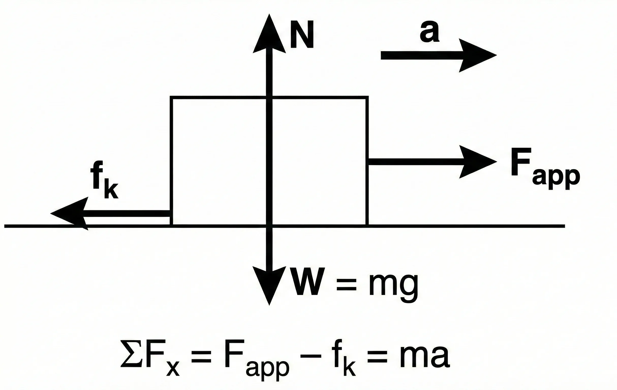
Block with kinetic friction on a horizontal surface
Scenario: A 15 kg block is pushed with a horizontal force of 80 N. Kinetic friction opposing motion is 26 N. Find the acceleration.
Step 1: Sum the forces in the horizontal direction.
Step 2: Apply Newton’s Second Law.
Result: The block accelerates at 3.6 m/s².
Interpretation: The correct answer comes from the net force, not the 80 N push alone. This is why force balance is the critical setup step.
Common mistakes, limits, and engineering checks
Newton’s Second Law is simple in form, but wrong answers usually come from force accounting errors, not algebra mistakes.
Common mistake: using an applied force instead of the net force
Many problems include friction, support reactions, drag, or multiple applied loads. The law uses the sum of all external forces, not just the largest visible force in the diagram.
Common mistake: confusing mass with weight
Mass is measured in kilograms and resists acceleration. Weight is a force equal to \(mg\). Mixing these two is one of the fastest ways to get unit errors and incorrect force balances.
Engineering check: does the acceleration direction make sense?
The computed acceleration should point in the same direction as the net force. If your result points opposite the summed force direction, revisit the sign convention or force balance.
Engineering check: define the system boundary first
Whether gravity, tension, or contact forces are internal or external depends on the chosen system. This is a small detail in basic physics, but it becomes a major engineering issue when multiple bodies or connected systems are involved.
A practical decision rule
- Use \(\sum F = ma\) for constant-mass bodies in most mechanics problems.
- Use component form when motion is not purely one-dimensional.
- Use impulse-momentum when force acts over a short time interval.
- Use the general momentum equation when mass flow or variable mass matters.
Newton’s Second Law FAQ
What is Newton’s Second Law in simple terms?
It states that the net force on an object equals its mass times its acceleration, so stronger net forces create greater acceleration and larger masses resist acceleration more.
What is the formula for Newton’s Second Law?
The most common form is \(\sum F = ma\), where \(\sum F\) is net force, \(m\) is mass, and \(a\) is acceleration.
What happens to acceleration if mass is doubled?
If net force stays the same and mass is doubled, acceleration is cut in half. That inverse relationship is one of the central ideas in Newton’s Second Law.
Is gravity an internal or external force in Newton’s Second Law?
It depends on the system boundary. If the Earth is outside the chosen system, gravity is an external force. If the Earth and object are treated as one combined system, gravity can be internal to that larger system.