
Key Takeaways
- Core idea: A Bode plot shows magnitude and phase versus frequency so engineers can see how a system responds to slow, moderate, and fast inputs.
- Engineering use: In control systems, Bode plots help estimate bandwidth, resonance, gain crossover, phase crossover, gain margin, and phase margin.
- What controls it: The plot shape comes from transfer function gain, poles, zeros, time constants, damping, delay, and the frequency range being evaluated.
- Practical check: Confirm whether the frequency axis is in rad/s or Hz and whether the plotted transfer function is open-loop or closed-loop.
Table of Contents
Introduction
Bode plots are frequency response graphs that show a system’s gain and phase shift across a range of frequencies. In control systems engineering, they help connect a transfer function to real design questions such as response speed, resonance, noise rejection, gain margin, phase margin, and closed-loop stability risk.
How to Read a Bode Plot at a Glance
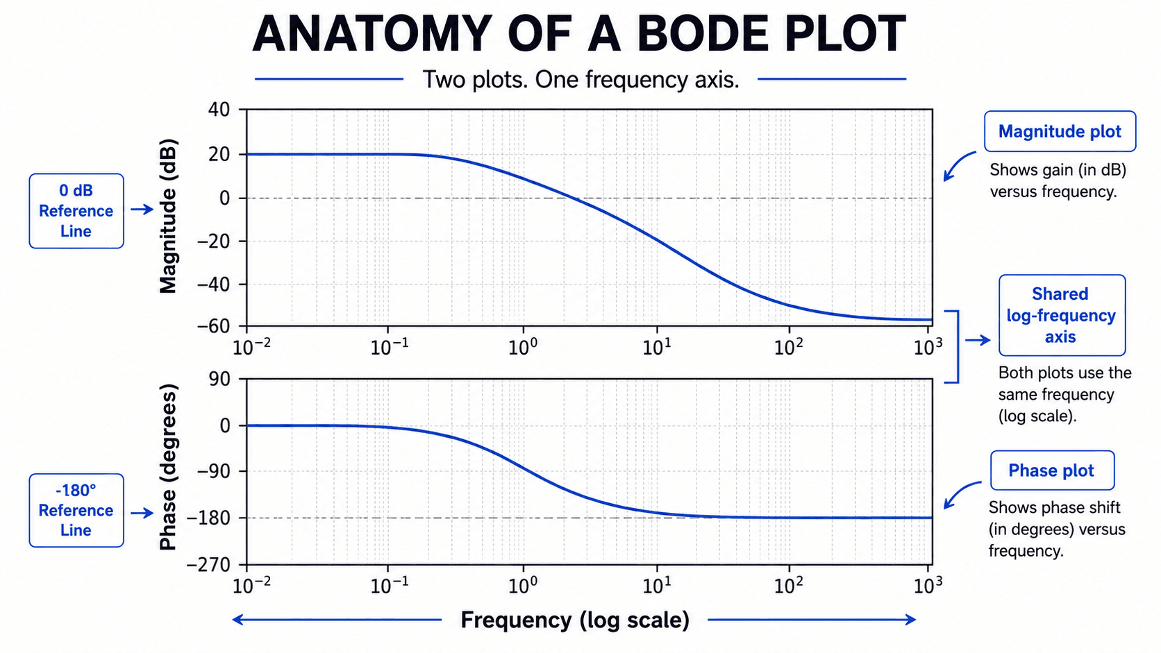
Start by reading the frequency axis, then compare the magnitude and phase at the same frequency. The 0 dB line and -180° phase line become especially important when evaluating feedback stability.
What Is a Bode Plot?
A Bode plot is a frequency-domain representation of a system’s transfer function. Instead of showing how output changes over time, it shows how the output amplitude and phase shift change as input frequency changes. This makes it especially useful for feedback control, filters, amplifiers, power electronics, and mechanical systems with dynamic behavior.
The most common form uses two stacked plots. The magnitude plot is usually shown in decibels, and the phase plot is usually shown in degrees. Both use a logarithmic frequency axis, which lets engineers view low-frequency behavior, crossover regions, and high-frequency roll-off on the same diagram.
In a control workflow, the Bode plot usually starts with a transfer function from system modeling. The plot then helps translate that model into design judgment: whether the system reacts quickly enough, rejects noise properly, and has enough separation from instability.
How to Interpret a Bode Plot
Interpreting a Bode plot means reading the magnitude and phase together. A frequency that looks acceptable on the magnitude plot may still be risky if the phase lag is too large. A fast-looking response may also amplify noise or excite resonance if the high-frequency behavior is not controlled.
Identify the frequency range, read the low-frequency gain, find the 0 dB crossover, check the phase at that same frequency, look for resonant peaks, confirm the final roll-off slope, and then evaluate gain margin and phase margin if the plot is being used for feedback stability.
| Step | What to inspect | Why it matters |
|---|---|---|
| 1. Frequency range | Check whether the x-axis is in rad/s or Hz and whether it covers the expected operating range. | A correct-looking curve can still be misleading if the axis units or frequency range are wrong. |
| 2. Low-frequency gain | Read the magnitude at the left side of the plot. | This often indicates tracking ability, disturbance rejection, or steady low-frequency amplification. |
| 3. Crossover region | Find where magnitude approaches or crosses 0 dB. | The gain crossover frequency is central to phase margin and closed-loop stability review. |
| 4. Phase at crossover | Read the phase angle at the gain crossover frequency. | Too much phase lag near crossover reduces stability margin and can lead to oscillation. |
| 5. Peaks and roll-off | Look for resonance peaks and the final high-frequency slope. | Peaks can indicate lightly damped modes, while roll-off affects noise amplification and response speed. |
Key Bode Plot Equations
Bode plots are built by evaluating a transfer function on the imaginary axis. The result is a complex value at each frequency, with a magnitude and an angle.
The factor 20 is used because Bode magnitude usually represents amplitude gain. Power ratios use \(10\log_{10}(\cdot)\), which is a common source of confusion when readers first learn decibels.
- \(G(s)\) Transfer function in the Laplace domain.
- \(G(j\omega)\) Frequency response evaluated at angular frequency \( \omega \).
- \( \omega \) Angular frequency in rad/s.
- \(f\) Frequency in Hz, related to angular frequency by \( f=\omega/(2\pi) \).
- 0 dB Unity amplitude gain, meaning output amplitude equals input amplitude at that frequency.
Magnitude, Phase, and the Log Frequency Axis
The magnitude plot answers the question: “How much does the system amplify or attenuate this frequency?” The phase plot answers a different question: “How much does the output lag or lead the input at this frequency?” Together, they show whether the system passes low frequencies, rejects high frequencies, resonates, delays the output, or risks instability when placed in feedback.
Why the frequency axis is logarithmic
Control systems often behave differently across several orders of magnitude. A motor drive, sensor filter, or feedback loop may need to show behavior from fractions of a radian per second to thousands of radians per second. A logarithmic axis compresses that range while preserving frequency ratios, which are more useful than equal frequency spacing for dynamic systems.
Why magnitude is shown in decibels
Decibels make multiplication easier to interpret visually. Gains, poles, and zeros combine as additive slope changes on the plot. A flat line means constant gain, a downward slope usually indicates roll-off, and a sharp peak may indicate resonance or lightly damped dynamics.
Why phase matters in feedback
Phase lag is one of the main reasons feedback systems become unstable. If a loop has high gain at a frequency where the output is nearly 180° out of phase with the input, negative feedback can effectively behave like positive feedback. This is why phase near crossover is more important than phase far away from crossover.
How Poles and Zeros Shape Bode Plots
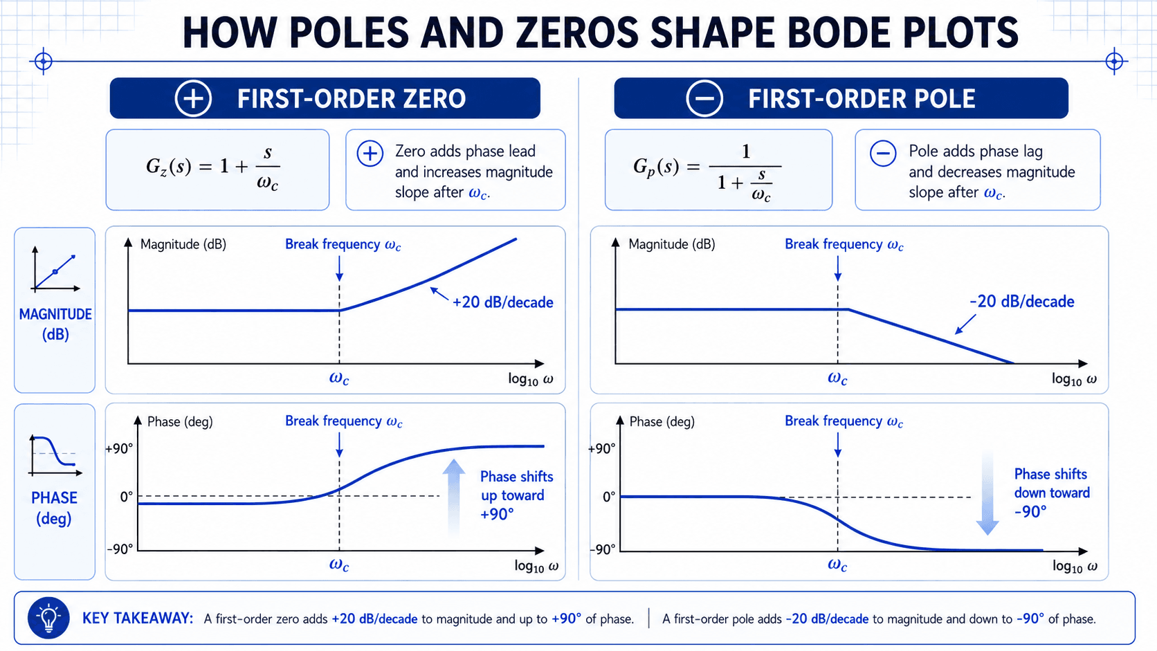
The shape of a Bode plot is mostly controlled by poles, zeros, and gain. In the figure below, focus on what happens after the break frequency. The zero increases slope and phase, while the pole decreases slope and phase.
Break frequency
The break frequency, often written as \( \omega_c \), is where a pole or zero begins to noticeably change the response. For a first-order term, the magnitude transition is gradual, not a perfectly sharp corner. The straight-line Bode sketch is an approximation used to understand the trend quickly.
Cumulative slope
Bode magnitude slope is cumulative. If a transfer function has two more poles than zeros at high frequency, the high-frequency magnitude slope will often trend toward -40 dB/decade. This simple check is one of the fastest ways to catch a missing pole, missing zero, or incorrectly simplified transfer function.
Minimum-phase and nonminimum-phase behavior
The common rule that a zero adds phase lead assumes a minimum-phase zero. A right-half-plane zero can increase magnitude like a zero while adding phase lag, which is one reason nonminimum-phase systems are harder to control.
| Transfer function feature | Magnitude effect | Phase effect |
|---|---|---|
| Constant gain | Moves the magnitude plot up or down without changing slope. | Usually no phase change if the gain is positive; negative gain adds phase inversion. |
| First-order zero | Adds about +20 dB/decade after the break frequency. | Adds phase lead, often approaching +90° for a minimum-phase zero. |
| First-order pole | Adds about -20 dB/decade after the break frequency. | Adds phase lag, often approaching -90° for a simple pole. |
| Second-order pole pair | Can create a resonant peak and a -40 dB/decade high-frequency trend. | Can add up to about -180° of phase lag depending on damping. |
| Time delay | Does not change magnitude by itself for an ideal delay. | Adds increasing phase lag as frequency increases. |
How to Draw a Bode Plot by Hand
Hand-sketching a Bode plot is not about replacing software. It is a control systems skill that helps engineers understand the dominant dynamics before trusting a generated plot. The workflow is especially useful for first-order systems, filters, compensators, and approximate stability checks.
Put the transfer function in standard form, identify gain, list every pole and zero, mark each break frequency, add magnitude slope changes, sketch the phase transitions, then compare the final low-frequency and high-frequency trends against the transfer function.
- Write the transfer function in standard form. Separate constant gain, first-order terms, second-order terms, integrators, and differentiators.
- Identify all break frequencies. Mark each pole and zero on the logarithmic frequency axis.
- Build the magnitude plot. Start with gain, then add slope changes at each break frequency.
- Build the phase plot. Add phase lead for zeros and phase lag for poles over the transition range.
- Check the trend. Confirm the high-frequency slope matches the net number of poles and zeros.
Before using a hand sketch for design judgment, verify the low-frequency gain, the high-frequency slope, and the phase direction. If any of those disagree with the transfer function structure, the plot is probably wrong.
Bode Plot Worked Example for a First-Order System
A simple first-order transfer function shows why Bode plots are useful. Consider a system with gain 10 and one pole at 5 rad/s:
Step 1: Find the low-frequency gain
At low frequency, the denominator is approximately 1, so the gain is about 10. In decibels:
The magnitude plot starts near 20 dB. This means the output amplitude is about 10 times the input amplitude at very low frequency.
Step 2: Mark the break frequency
The denominator term \(1+s/5\) gives a break frequency of \( \omega_c=5 \text{ rad/s} \). Near this frequency, the magnitude begins transitioning from flat behavior to a downward slope.
Step 3: Apply the pole slope
A first-order pole contributes approximately -20 dB/decade after the break frequency. One decade above 5 rad/s, around 50 rad/s, the asymptotic magnitude estimate is about 20 dB lower than the low-frequency level.
Step 4: Interpret the phase
The phase starts near 0° at low frequency, passes through about -45° near the break frequency, and trends toward -90° at high frequency. In engineering terms, the system follows slow inputs well but increasingly lags and attenuates faster inputs.
This first-order response behaves like a low-pass system: low-frequency inputs pass with gain, while high-frequency inputs are increasingly attenuated and delayed.
Bode Plots for Filters and Frequency Response
Bode plots are widely used to understand filters because filters are defined by how they treat different frequencies. The same plot format used in feedback control is also useful for RC filters, active filters, sensor filtering, audio systems, signal conditioning, and power electronics.
| Filter behavior | Typical Bode plot pattern | Engineering meaning |
|---|---|---|
| Low-pass filter | Magnitude is relatively flat at low frequency and rolls off after cutoff. | Slow signals pass, while high-frequency noise or ripple is reduced. |
| High-pass filter | Magnitude is low at low frequency and rises toward a pass band. | DC or slow drift is rejected while faster changes pass through. |
| Band-pass filter | Magnitude peaks or remains high over a middle frequency range. | A selected frequency band is emphasized while lower and higher frequencies are rejected. |
| Resonant system | Magnitude has a peak near a natural frequency. | The system may amplify inputs near that frequency, increasing vibration, overshoot, or oscillation risk. |
For many first-order filters, cutoff frequency is associated with the -3 dB point, where the output amplitude is about 70.7% of the pass-band value. In higher-order or resonant systems, cutoff and bandwidth require more careful interpretation.
Using Bode Plots for Stability Margins
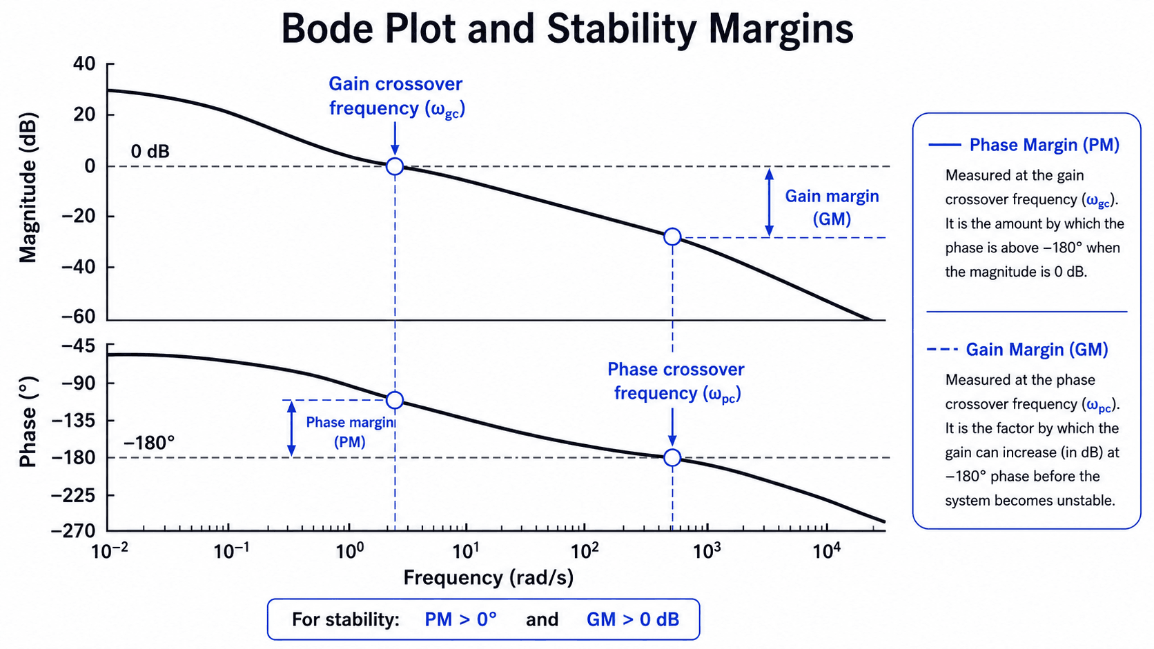
In feedback control, Bode plots are often used on the open-loop transfer function to estimate how close the closed-loop system is to instability. The figure below highlights the two crossover points that matter most: gain crossover and phase crossover.
Gain crossover frequency
The gain crossover frequency is where the open-loop magnitude crosses 0 dB, or \( |G(j\omega)|=1 \). At this frequency, the phase value tells you how much additional phase lag remains before the system reaches -180°. That difference is the phase margin.
Phase crossover frequency
The phase crossover frequency is where the phase reaches -180°. At that frequency, the magnitude value tells you how much gain can increase before the magnitude reaches 0 dB at the critical phase condition. That difference is the gain margin.
Multiple crossover frequencies
Higher-order systems can have more than one gain crossover or phase crossover. When that happens, engineers must evaluate the most critical crossover region rather than assuming one margin value tells the full story.
A positive phase margin and gain margin indicate separation from the basic instability boundary, but practical control designs normally require additional margin for modeling error, time delay, sensor noise, actuator limits, and operating variation.
What Engineers Look for in a Bode Plot
A useful Bode plot is not just a curve on a graph. Engineers read it as a design review tool. The key question is whether the response supports the required performance without creating noise problems, resonance problems, actuator problems, or stability risk.
| Feature on the Bode plot | What to look for | Engineering implication |
|---|---|---|
| Low-frequency gain | Magnitude level at the left side of the plot. | Shows how strongly the system responds to slow commands or disturbances. |
| Bandwidth | Frequency range where the system still responds strongly. | Relates to speed of response, tracking ability, and disturbance rejection. |
| Resonant peak | A bump or sharp rise in magnitude before roll-off. | May indicate lightly damped dynamics, overshoot risk, vibration, or sensitivity to excitation near that frequency. |
| High-frequency roll-off | Magnitude decreasing at high frequency. | Can help reduce noise amplification but may also limit fast response. |
| Phase lag near crossover | Phase angle when magnitude approaches 0 dB. | Directly affects phase margin and closed-loop stability risk. |
| Time delay | Phase decreasing faster as frequency increases. | Can reduce stability margin even when the magnitude plot appears acceptable. |
This is where Bode plots become more than classroom diagrams. The same magnitude roll-off that protects a system from high-frequency noise can also slow command following. The same bandwidth increase that improves response speed can reduce phase margin if the controller pushes crossover into a region with too much lag.
Bode Plot Sanity Check Table
Use this review table before trusting a plotted result, especially when the plot came from software, a simplified model, or a hand sketch. Most serious Bode plot mistakes are not drawing errors; they are model, unit, or interpretation errors.
| Check | What to look for | Why it matters |
|---|---|---|
| Transfer function type | Confirm whether the plot is open-loop, closed-loop, plant-only, or controller-only. | Stability margins are normally interpreted from the open-loop response, not just any transfer function. |
| Frequency units | Check whether the x-axis is rad/s or Hz. | A unit mismatch can shift crossover and bandwidth interpretation by a factor of \(2\pi\). |
| Low-frequency gain | Compare the starting magnitude to the transfer function’s DC gain when it exists. | This catches wrong gain constants, sign mistakes, and scaling errors. |
| High-frequency slope | Compare the final slope to the net number of poles minus zeros. | A slope mismatch often means a pole, zero, or integrator was missed. |
| Phase direction | Confirm that poles add lag and zeros add lead unless nonminimum-phase behavior is present. | Incorrect phase direction can completely reverse a stability conclusion. |
| Margin values | Identify gain crossover and phase crossover before quoting phase margin or gain margin. | Margins without the correct crossover points can be misleading or meaningless. |
| Software output | Check whether phase is wrapped, unwrapped, displayed in degrees, or displayed in radians. | Display settings can change the visual interpretation even when the underlying response is the same. |
Bode Plot vs Nyquist Plot vs Root Locus
Bode plots, Nyquist plots, and root locus plots are related control-system tools, but they answer different questions. A strong design review often uses more than one of them.
| Method | What it shows | Best use |
|---|---|---|
| Bode plot | Magnitude and phase versus frequency. | Evaluating bandwidth, frequency response, gain margin, phase margin, and noise sensitivity. |
| Nyquist plot | Complex frequency response in the real-imaginary plane. | Evaluating stability using encirclement logic, especially when Bode margins are not enough. |
| Root locus | Closed-loop pole movement as gain changes. | Understanding how gain affects closed-loop pole locations, damping, and response speed. |
Bode plots are usually the most intuitive starting point for frequency-domain design. Nyquist analysis becomes important when encirclement and robustness need closer review, while root locus is useful when the main question is how closed-loop poles move as gain changes.
When This Breaks Down
Bode plots are most reliable when the system can be represented as a linear time-invariant model over the frequency range of interest. The farther the real system gets from that assumption, the more carefully the plot must be interpreted.
- Nonlinear behavior: Saturation, deadband, backlash, friction, and switching behavior can make frequency response depend on input amplitude.
- Time-varying systems: If plant dynamics change with operating point, speed, temperature, or loading, one Bode plot may not represent all conditions.
- Transport delay: Delay adds phase lag that can reduce phase margin even when the magnitude plot looks acceptable.
- Unmodeled high-frequency dynamics: Sensors, actuators, filters, flexible modes, and sampling effects may appear outside the original model.
- Nonminimum-phase zeros: Right-half-plane zeros can create counterintuitive phase behavior and limit achievable control performance.
- Multiple crossover regions: A single quoted gain margin or phase margin can hide another more critical crossover.
A clean Bode plot from a simplified model can still be unsafe to use for final controller tuning if actuator limits, sensor noise, delay, saturation, or flexible modes were omitted from the model.
Common Mistakes and Practical Checks
Most Bode plot errors happen because the graph is read without checking the model behind it. The visual format is simple, but the interpretation depends on units, transfer function form, and whether the plotted response is the correct one for the engineering question.
- Confusing Hz and rad/s: The curve shape may look the same, but crossover frequency, bandwidth, and tuning conclusions can be wrong.
- Reading 0 dB as zero output: 0 dB means unity gain, not no response.
- Ignoring phase wrapping: Software may display phase with jumps or wrapped angles, which can confuse phase margin interpretation.
- Forgetting cumulative slope: Each pole and zero contributes to the final magnitude slope; isolated slope rules must be combined.
- Using closed-loop plots for open-loop margins: Gain and phase margins are usually based on open-loop loop gain, not the closed-loop response.
- Treating positive margins as a finished design: Positive margins are a starting check, not a complete guarantee of acceptable transient response or robustness.
Before reporting gain margin or phase margin, state the plotted transfer function, the frequency units, and the crossover frequencies. That single habit prevents many control review errors.
Useful References and Software Context
Bode plots are often generated with analysis software, but the engineering value comes from understanding what the plotted magnitude and phase mean. Software documentation is useful for confirming how frequency response data is computed, displayed, and customized.
- MathWorks Control System Toolbox: Bode frequency response of dynamic system explains how MATLAB computes and returns magnitude, phase, and frequency data for dynamic system models.
- Engineering use: Software-generated plots should be reviewed against the transfer function structure, expected pole-zero behavior, units, and stability margin definitions.
- Design context: In real control work, Bode plots are usually used alongside stability analysis, time response checks, model validation, actuator limits, sensor noise review, and controller tuning.
Frequently Asked Questions
A Bode plot is used to study how a linear system responds to different input frequencies. In control systems engineering, it helps engineers estimate gain, phase lag, bandwidth, resonance, and stability margins without solving the full time response for every possible input.
A Bode plot is one way to display frequency response. Frequency response describes how a system behaves as input frequency changes; a Bode plot shows that behavior as magnitude and phase on logarithmic frequency axes.
On a Bode magnitude plot, 0 dB means unity gain. The output amplitude is equal to the input amplitude at that frequency. It does not mean zero output or zero signal.
A first-order zero generally increases the magnitude slope by 20 dB per decade after its break frequency and adds phase lead. A first-order pole generally decreases the magnitude slope by 20 dB per decade after its break frequency and adds phase lag.
Phase margin is read at the gain crossover frequency, where the magnitude plot crosses 0 dB. Gain margin is read at the phase crossover frequency, where the phase reaches -180 degrees. Together, they estimate how close the open-loop system is to closed-loop instability.
Summary and Next Steps
Bode plots show how a system’s magnitude and phase change with frequency. For control systems engineering, they are one of the most useful ways to connect transfer function structure to bandwidth, resonance, crossover frequency, and stability margin.
The most important practical checks are simple: know which transfer function is being plotted, confirm rad/s versus Hz, identify poles and zeros, check the expected slope, and read phase margin and gain margin at the correct crossover frequencies.
Where to go next
Continue your learning path with related Turn2Engineering resources.
-
Control Theory
Build the foundation behind feedback, transfer functions, stability, and frequency-domain design.
-
Stability Analysis
Learn how frequency-domain and time-domain methods are used to judge whether a control system remains stable.
-
Root Locus Method
See how pole locations move as gain changes and how root locus complements Bode plot design.