Key Takeaways
- Core idea: Load flow analysis calculates the steady-state operating point of a power system, including bus voltages, angles, real power, reactive power, equipment loading, and losses.
- Engineering use: Engineers use load flow studies to check voltage profiles, overloaded lines or transformers, reactive power support, generation dispatch, feeder limits, and expansion scenarios.
- What controls it: Results depend on bus types, load assumptions, generator voltage setpoints, line and transformer impedances, transformer taps, shunt devices, per-unit bases, and reactive power limits.
- Practical check: A converged load flow is not automatically acceptable; voltage limits, thermal ratings, losses, reactive capability, and model assumptions still need engineering review.
Table of Contents
Introduction
Load flow analysis is a steady-state power system study that calculates bus voltages, voltage angles, real and reactive power flow, equipment loading, and system losses for a specified operating condition. Engineers use it to check whether a transmission network, distribution feeder, substation, facility, or renewable interconnection can operate within voltage and thermal limits.
Load Flow Study Workflow
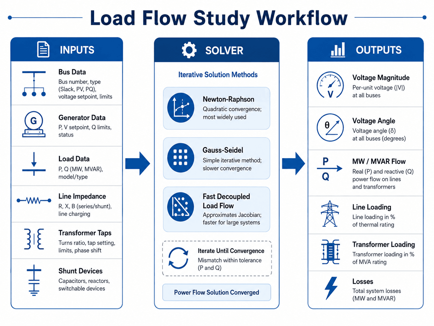
The most important idea is that load flow analysis is not just a calculation. It is a modeling workflow: define the system, solve the steady-state operating point, then decide whether the result is electrically acceptable.
What Is Load Flow Analysis?
Load flow analysis, also called power flow analysis, determines how real power \(P\) and reactive power \(Q\) move through an electrical network under a selected operating case. It solves for unknown bus voltages and phase angles while reporting line flows, transformer loading, voltage drop, reactive support, and losses.
In a power system model, buses represent connection points such as generators, substations, switchgear, load centers, distribution nodes, or interconnection points. Lines, transformers, shunt capacitors, reactors, and loads connect those buses. The practical question is simple: under the assumed load and generation condition, does the system operate within acceptable voltage and thermal limits?
Load flow analysis is normally the base study for other power system work. Fault studies, voltage regulation studies, stability studies, contingency analysis, interconnection studies, and equipment upgrade decisions often start from a trusted steady-state operating case.
Basic load flow glossary
These terms appear throughout load flow studies and software output reports.
| Term | Meaning in load flow analysis | Why it matters |
|---|---|---|
| Bus | A node where generators, loads, lines, transformers, or shunt devices connect. | Bus voltage magnitude and angle are central solved quantities. |
| Branch | A line, cable, or transformer connecting two buses. | Branch flows determine loading, voltage drop, and losses. |
| Injection | Net generation minus load at a bus. | Positive injection usually represents power entering the network; negative injection usually represents load consumption. |
| Mismatch | The difference between specified and calculated real or reactive power during iteration. | Convergence is reached when mismatch is reduced below the selected tolerance. |
| Slack bus | The reference bus that balances losses and model mismatch. | It anchors the voltage angle reference and absorbs the remaining power balance. |
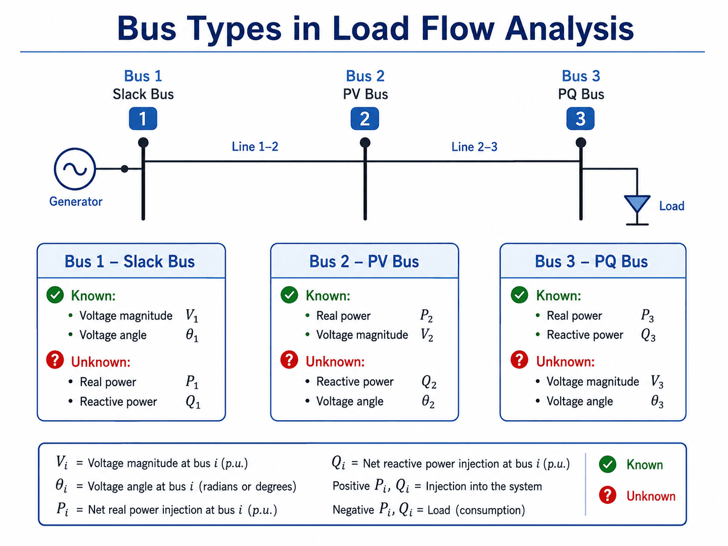
Bus Types in Load Flow Analysis
Load flow analysis works by assigning known and unknown quantities to each bus. The solver calculates the missing quantities so that real and reactive power balance across the network. The three most important bus types are the slack bus, PV bus, and PQ bus.
| Bus type | Known quantities | Unknown quantities | Engineering meaning |
|---|---|---|---|
| Slack bus | Voltage magnitude \(V\) and voltage angle \(\theta\) | Real power \(P\) and reactive power \(Q\) | Provides the reference angle and balances system losses and mismatch in the solved case. |
| PV bus | Real power \(P\) and voltage magnitude \(V\) | Reactive power \(Q\) and voltage angle \(\theta\) | Usually represents a generator, inverter, or voltage-controlled bus with a target voltage setpoint. |
| PQ bus | Real power \(P\) and reactive power \(Q\) | Voltage magnitude \(V\) and voltage angle \(\theta\) | Usually represents a load bus where demand is specified and voltage is solved. |
Why PV buses can become PQ buses
A PV bus is voltage-controlled only within the reactive capability of the generator, inverter, or voltage-control device. If the calculated \(Q\) exceeds the available reactive limit, the voltage setpoint is no longer physically achievable. In many load flow programs, the bus is then treated as a PQ bus with \(Q\) fixed at the limit, and the voltage magnitude becomes a solved result.
Load Flow Inputs and Outputs
A load flow model is built from equipment data and operating assumptions. The solver does not know whether the assumptions are realistic; it only solves the network described by the data. That makes input review one of the most important parts of the study.
| Model item | Typical data required | Why it matters in the result |
|---|---|---|
| Bus data | Bus number, nominal voltage, bus type, voltage setpoint, voltage limits | Defines the electrical nodes where voltages, angles, and injections are solved. |
| Load data | MW, MVAR, load model, power factor, operating scenario, diversity assumptions | Controls voltage drop, reactive demand, branch loading, and losses. |
| Generator data | MW output, voltage setpoint, reactive power limits, operating status | Controls power injection, voltage support, and reactive reserve. |
| Line and cable data | Resistance, reactance, charging susceptance, ampacity or thermal rating | Controls power transfer, voltage drop, losses, and line loading. |
| Transformer data | Impedance, MVA rating, winding voltages, tap position, phase shift | Controls voltage transformation, reactive behavior, and loading across voltage levels. |
| Shunt devices | Capacitor banks, reactors, switching status, MVAR rating | Affects voltage profile and reactive power balance at nearby buses. |
Typical load flow outputs
Output normally includes bus voltage magnitude, bus voltage angle, generator real and reactive output, line and transformer MW/MVAR flow, current, percent loading, and system losses. The most useful output is not just a table of numbers; it is the engineering interpretation of which buses are weak, which branches are overloaded, and which corrective actions are available.
Why per-unit values are used
Power systems often include multiple voltage levels connected through transformers. The per-unit system normalizes voltage, current, impedance, and power values to selected base quantities, making it easier to compare equipment and solve networks with different voltage levels. Per-unit data also helps engineers spot abnormal impedances or voltage results more quickly.
Core Load Flow Equations
Load flow analysis is based on AC circuit relationships, complex power, and the bus admittance matrix. Most practical studies are solved by software, but understanding the equations helps explain why voltage magnitude, angle, real power, and reactive power are coupled.
The complex power injected at bus \(i\) is related to the bus voltage \(V_i\) and the complex conjugate of current \(I_i\). A positive power injection typically represents generation into the network, while a negative injection typically represents load consumption.
The \(Y_{bus}\) matrix represents how buses are electrically connected through line, transformer, and shunt admittances. Diagonal terms collect the admittances connected to a bus, while off-diagonal terms represent the electrical coupling between buses. The load flow solver iterates until the real and reactive power mismatches are within tolerance.
- \(V_i\) Voltage magnitude and angle at bus \(i\), usually expressed in per unit and degrees.
- \(P_i\) Net real power injection at bus \(i\), commonly reported in MW or per unit.
- \(Q_i\) Net reactive power injection at bus \(i\), commonly reported in MVAR or per unit.
- \(Y_{ik}\) Admittance matrix term connecting bus \(i\) and bus \(k\), based on equipment impedance and shunt data.
Worked Example: Simple 3-Bus Load Flow Setup
A useful beginner load flow example is a three-bus system with one slack bus, one generator bus, and one load bus. The point is not to hand-calculate every iteration, but to understand what is specified, what is solved, and how the final result is judged.
| Bus | Type | Specified values | Solver calculates |
|---|---|---|---|
| Bus 1 | Slack | \(V = 1.04\) p.u., \(\theta = 0^\circ\) | Real power \(P\) and reactive power \(Q\) |
| Bus 2 | PV | \(P = 100\) MW, \(V = 1.02\) p.u. | Reactive power \(Q\) and voltage angle \(\theta\) |
| Bus 3 | PQ | \(P = 80\) MW, \(Q = 35\) MVAR | Voltage magnitude \(V\) and voltage angle \(\theta\) |
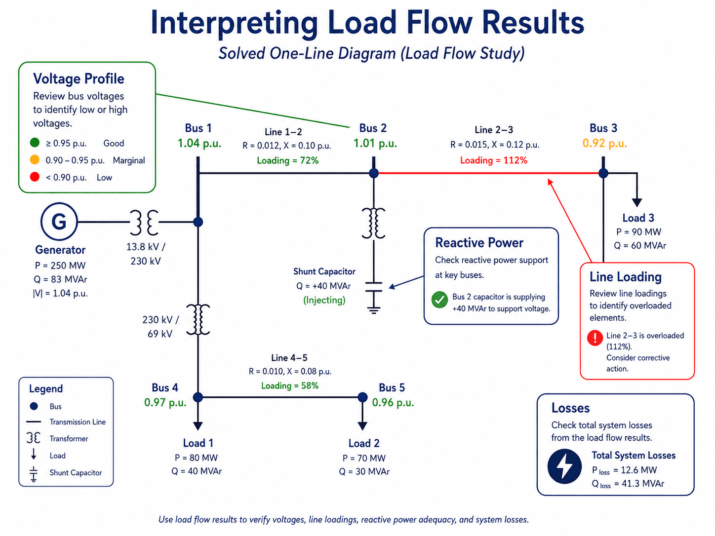
How to read the solved result
If Bus 3 solves at \(0.92\) p.u., the engineer should review whether that voltage is acceptable for the project criteria. If Line 2–3 solves at 112% loading, the case fails on thermal loading even if every bus voltage appears acceptable. This is why load flow interpretation must include voltage, loading, reactive output, and losses together.
The solver answers the equations, but the engineer decides whether the case passes. A converged 3-bus case with low voltage or an overloaded line still requires corrective action.
Load Flow Solution Methods
Load flow equations are nonlinear, so the solution is normally found with an iterative numerical method. The best method depends on system size, model quality, convergence behavior, and the type of study being performed.
| Method | Best use | Strength | Limitation |
|---|---|---|---|
| Gauss-Seidel | Small systems, teaching examples, simple demonstrations | Conceptually straightforward and easy to follow step by step. | Can converge slowly and may struggle with large or stressed systems. |
| Newton-Raphson | Most practical engineering studies and larger systems | Strong convergence behavior and widely used in power system software. | Requires forming and updating a Jacobian matrix, which is more computationally involved. |
| Fast Decoupled Load Flow | Large transmission systems where assumptions are reasonable | Faster for many large systems because it simplifies the coupling between \(P\), \(Q\), voltage, and angle. | Less suitable when resistance is high, voltage conditions are weak, or assumptions are not valid. |
Method selection guide
| Study situation | Preferred approach | Reason |
|---|---|---|
| Small teaching problem | Gauss-Seidel | Easy to demonstrate the iterative logic without hiding the process. |
| General engineering study | Newton-Raphson | Reliable convergence behavior and broad support in commercial software. |
| Large transmission planning case | Fast Decoupled Load Flow | Efficient when decoupling assumptions are reasonable. |
| Weak distribution system or high R/X feeder | Newton-Raphson or specialized distribution power flow | Fast decoupled assumptions may be less accurate when resistance is significant. |
| Case with convergence problems | Review model data before changing methods | Non-convergence often points to bad data, topology errors, or a stressed operating condition. |
Convergence does not prove the model is correct. A solver can converge on a bad model if the input data is wrong, the operating scenario is unrealistic, or equipment limits are ignored.
How Engineers Interpret Load Flow Results
The solved load flow case gives engineers a snapshot of the system operating point. The next step is to review whether the calculated voltages, flows, and losses are acceptable for the project objective, operating scenario, and equipment ratings.
| Result to review | What to look for | Engineering implication |
|---|---|---|
| Voltage profile | Buses with high, low, or marginal per-unit voltage | May indicate voltage drop, weak reactive support, incorrect tap settings, or poor load assumptions. |
| Line loading | Lines operating near or above thermal rating | May require dispatch changes, reconfiguration, conductor upgrades, or contingency review. |
| Transformer loading | Percent of MVA rating and overload margin | May control expansion plans, tap settings, cooling requirements, or operating limits. |
| Reactive power flow | Large MVAR demand, generator Q limits, capacitor contribution | Often controls voltage support, generator capability, and local reactive compensation needs. |
| System losses | MW losses, MVAR losses, and high-loss branches | Useful for efficiency studies, planning comparisons, and evaluating alternative operating cases. |
What a good load flow result looks like
| Output | Healthy sign | Needs review |
|---|---|---|
| Bus voltage | Most buses remain within the project’s expected operating range. | Buses near limits, outside criteria, or unexpectedly high after tap or capacitor changes. |
| Line loading | Branches remain below normal and emergency ratings for the scenario. | Any line near or above rating, especially under contingency or future-load cases. |
| Transformer loading | Transformer loading stays within nameplate or approved operating criteria. | Overload, unexpected reverse flow, or excessive loading after network reconfiguration. |
| Reactive power | Generators, inverters, capacitors, and reactors provide adequate local support. | Generator or inverter Q limits exceeded, weak voltage support, or large reactive transfers. |
| Slack bus output | Slack bus absorbs a reasonable mismatch and system loss balance. | Unrealistic slack output, which may signal missing load, bad generation dispatch, or data errors. |
Load Flow Analysis in Power System Software
Load flow studies are commonly performed in tools such as ETAP, PowerWorld, PSS/E, DIgSILENT PowerFactory, OpenDSS, MATLAB-based tools, and Python libraries such as pandapower. The software may differ, but the engineering workflow is similar.
| Workflow step | What the engineer does | What to verify |
|---|---|---|
| Build the one-line model | Create buses, lines, transformers, generators, loads, breakers, and shunt devices. | Topology matches drawings, field status, and the study case. |
| Enter electrical data | Add impedance, ratings, tap positions, voltage bases, load data, and generator limits. | Data is on the correct base and reflects current equipment settings. |
| Assign bus types | Set slack, PV, and PQ buses according to the operating role. | Voltage-control buses have realistic reactive limits. |
| Select the operating case | Run peak, light-load, future expansion, DER export, or outage scenarios as needed. | The scenario answers the actual engineering question. |
| Run the solver | Use Newton-Raphson or another appropriate method until mismatch tolerance is met. | Convergence is achieved without hiding model warnings or limit violations. |
| Review outputs | Check voltage, line loading, transformer loading, generator Q, losses, and alerts. | The solved case meets project criteria, not just mathematical convergence. |
Modern systems with solar, batteries, and inverter-based generation may require special attention to export conditions, reactive power capability, voltage control mode, and reverse power flow. A case that looks normal at peak load can behave very differently during light load with high distributed generation output.
Load Flow Model Review Checklist
The most valuable load flow study is not the one with the most detailed output table; it is the one with a model that has been reviewed carefully enough to trust. Use the checklist below before relying on the results for planning, operation, or design decisions.
Build the network model, confirm base values, assign bus types, enter load and generation assumptions, solve the case, review convergence, check voltage and loading limits, then run the scenarios that actually matter: peak load, light load, future expansion, generation changes, switching changes, DER export, and outage cases where relevant.
| Review check | What to look for | Why it matters |
|---|---|---|
| System base values | Correct MVA base and voltage bases for each zone or voltage level | Wrong per-unit bases can distort impedances, flows, and voltage drops throughout the model. |
| Bus type assignments | Slack, PV, and PQ buses assigned according to the actual operating role | Wrong bus types can force unrealistic voltage control or hide reactive power problems. |
| Transformer data | Correct winding voltages, impedance, MVA rating, tap position, and phase shift | Transformer errors can produce misleading voltage profiles and loading results. |
| Generator reactive limits | Q limits, voltage setpoints, operating status, and PV-to-PQ behavior | Reactive limits often control whether a voltage target is physically achievable. |
| Load assumptions | Peak load, light load, diversity, power factor, and load model type | Voltage drop, losses, and equipment loading can change significantly with scenario selection. |
| Connectivity and islanding | Disconnected buses, open breakers, unintended islands, or missing ties | Connectivity errors are a common cause of non-convergence or unrealistic results. |
| Equipment ratings | Line ampacity, transformer MVA rating, cable limits, and emergency ratings | A solved load flow case may still fail if branches or transformers exceed acceptable loading limits. |
Troubleshooting a Load Flow That Will Not Converge
Non-convergence is not just a software annoyance. It is often a clue that the model has bad data, unrealistic assumptions, disconnected equipment, insufficient reactive power support, or an operating point close to voltage instability.
| Symptom | Likely cause | Practical check |
|---|---|---|
| Solver diverges immediately | Bad input data, missing slack bus, or isolated island | Check topology, open breakers, bus connectivity, and reference bus assignment. |
| Voltage collapses in one area | Heavy loading, weak source, or insufficient reactive support | Review MVAR demand, capacitor status, generator Q limits, and transformer taps. |
| Generator exceeds reactive limit | Voltage setpoint is too aggressive or local support is weak | Check PV-to-PQ switching and available reactive capability. |
| Extremely high branch flow | Incorrect impedance, tap, rating, or topology | Verify line and transformer data against drawings, nameplates, and field status. |
| Case converges only with loose tolerance | Weak model, stressed case, or unresolved data issue | Investigate mismatch locations instead of accepting an artificially loose solution. |
Load Flow vs Fault Analysis, Short-Circuit Analysis, and Stability Studies
Load flow analysis is sometimes confused with other power system studies. The difference is the operating condition being studied and the type of result required. Load flow focuses on normal or planned steady-state operation, while fault and stability studies examine abnormal or time-dependent behavior.
| Study type | Primary question | Typical outputs | How it relates to load flow |
|---|---|---|---|
| Load flow analysis | Can the system operate acceptably under this load and generation condition? | Bus voltage, angle, MW/MVAR flow, loading, losses | Establishes the steady-state operating case. |
| Short-Circuit Analysis | How much fault current flows during abnormal low-impedance faults? | Fault current, device duty, interrupting requirements | Uses system impedance data but solves a different abnormal condition. |
| Fault analysis | How does the system behave during different fault types and fault locations? | Fault currents, voltage depression, sequence quantities | Often follows a base system model created for normal operating studies. |
| Stability analysis | Can the system remain synchronized after a disturbance? | Rotor angle behavior, frequency, dynamic voltage response | Often starts from a solved load flow operating point. |
| Optimal power flow | What operating point best meets an objective while satisfying constraints? | Optimized dispatch, losses, costs, voltages, flows, or constraint results | Builds on power flow equations but adds an optimization objective. |
For related background, see Power Systems Engineering and Voltage Regulation.
Engineering Judgment and Field Reality
Real load flow studies are scenario-dependent. A base case may pass, while a peak-load case, light-load case, contingency case, generator outage case, future expansion case, or distributed energy export case may reveal low voltage or overloaded equipment.
Field data can also differ from design data. Transformer taps may not match drawings, capacitor banks may be out of service, feeder loading may be unbalanced, and actual power factor may differ from assumed values. In distribution systems with solar, battery storage, or distributed generation, reverse power flow can change the expected voltage pattern.
A clean one-line diagram can hide the biggest source of error: stale operating assumptions. Before trusting the results, confirm that load levels, switching status, tap positions, generator dispatch, inverter control mode, and reactive devices match the actual scenario being studied.
Where Load Flow Analysis Breaks Down
Load flow analysis is powerful, but it is not a complete representation of all power system behavior. It is a steady-state study, so it does not directly show transient fault behavior, protective relay timing, dynamic stability, harmonics, frequency response, motor starting, arc flash, relay coordination, or switching transients.
- Dynamic disturbances: Load flow does not show rotor angle swings, frequency excursions, motor acceleration, or transient voltage recovery.
- Protection behavior: Load flow does not determine relay operation, breaker clearing time, or interrupting duty.
- Bad input data: A model with wrong impedances, ratings, loads, or tap settings can produce confident-looking but unreliable results.
- Unbalanced systems: Standard positive-sequence load flow may not capture severe phase imbalance unless the model and solver support unbalanced or three-phase analysis.
- Reactive power limits: Ignoring generator or inverter Q limits can make voltage control look better than it is in the field.
Common Load Flow Mistakes and Practical Checks
Load flow mistakes usually come from modeling assumptions rather than arithmetic. The most useful checks confirm that the electrical model resembles the actual system and that the solved case is meaningful for the decision being made.
| Common mistake | Why it matters | Practical check |
|---|---|---|
| Using the wrong load case | Peak, light-load, emergency, and future expansion cases can produce different voltage and loading results. | Run the scenario that matches the design or operating question. |
| Ignoring transformer taps | Tap settings strongly affect voltage profile, especially across voltage levels and long feeders. | Confirm actual tap positions and test whether tap changes create other voltage issues. |
| Treating convergence as approval | A converged case may still contain low voltage, overloads, unrealistic reactive output, or excessive losses. | Review voltage, loading, reactive limits, and losses after every solve. |
| Forgetting reactive power limits | Generator and inverter reactive capability can limit voltage support. | Check Q-limit violations and PV-to-PQ bus behavior. |
| Skipping contingency cases | A system that passes with all equipment in service may fail when a line, transformer, or generator is unavailable. | Run outage cases where reliability or planning criteria require them. |
Do not stop at “the load flow converged.” Review voltage limits, equipment loading, generator reactive output, transformer taps, scenario assumptions, and model warnings before using the result to support an engineering decision.
Engineering References and Design Guidance
Load flow study requirements depend on the system type, owner criteria, software model, project stage, and study purpose. Industrial, commercial, utility, and renewable-energy projects may each require different assumptions, reporting formats, and scenario reviews.
- IEEE recommended practice: IEEE Recommended Practice for Conducting Load-Flow Studies and Analysis of Industrial and Commercial Power Systems is a directly relevant reference for formal industrial and commercial power system load-flow study guidance, including steady-state power flow, voltage analysis, model validation, and how load-flow results support electrical design decisions.
- Project-specific criteria: Owner requirements, utility interconnection rules, equipment ratings, operating limits, and local design practices may control what voltage range, loading margin, or contingency performance is acceptable.
- Engineering use: Engineers use references and project criteria to decide which scenarios to study, which assumptions to document, and how to judge whether voltage, loading, losses, and reactive power support are acceptable.
Frequently Asked Questions
Load flow analysis is a steady-state power system study used to calculate bus voltages, voltage angles, real and reactive power flows, equipment loading, and system losses for a selected operating condition.
In most power engineering contexts, load flow analysis and power flow analysis refer to the same steady-state study. Power flow is technically more precise because the study tracks real and reactive power through the network, not just the connected loads.
The common methods are Gauss-Seidel, Newton-Raphson, and Fast Decoupled Load Flow. Newton-Raphson is widely used for larger engineering studies because it usually converges more reliably and quickly than basic iterative methods.
A load flow study can fail to converge because of bad model data, disconnected islands, unrealistic loading, poor initial voltage assumptions, incorrect transformer taps, reactive power limit violations, or a system operating close to voltage instability.
Load flow analysis solves the operating condition for a specified set of loads, generation, and network settings. Optimal power flow adds an optimization objective, such as minimizing cost, losses, or constraint violations, while still satisfying power flow equations and operating limits.
Summary and Next Steps
Load flow analysis is one of the core studies in power systems engineering because it shows how a network operates under a defined steady-state condition. It calculates bus voltages, voltage angles, MW and MVAR flows, line and transformer loading, and system losses.
The most useful load flow study combines accurate model data, appropriate bus types, reasonable operating scenarios, solver convergence review, and practical interpretation of voltage, loading, reactive power, and losses. A solved model is only valuable when the assumptions and engineering checks are sound.
Where to go next
Continue your learning path with related Turn2Engineering resources.
-
Voltage Regulation
Learn how voltage is controlled in power systems and why voltage profiles are a key load flow output.
-
Short-Circuit Analysis
Compare steady-state load flow studies with fault-current studies used for equipment duty and protection review.
-
Power System Efficiency
Explore how system losses, power factor, and operating conditions affect the efficiency of power delivery.