Key Takeaways
- Definition: Maxwell’s Equation refers to the equations that govern electric fields, magnetic fields, charge, current, and electromagnetic induction.
- Main use: Engineers use Maxwell’s equations to understand antennas, motors, transformers, transmission lines, shielding, capacitors, inductors, and electromagnetic waves.
- Watch for: The equations are field equations, so geometry, boundary conditions, material properties, frequency, and simplifying assumptions matter.
- Outcome: You will understand what each Maxwell equation says, what the variables mean, and when lumped circuit assumptions stop being enough.
Table of Contents
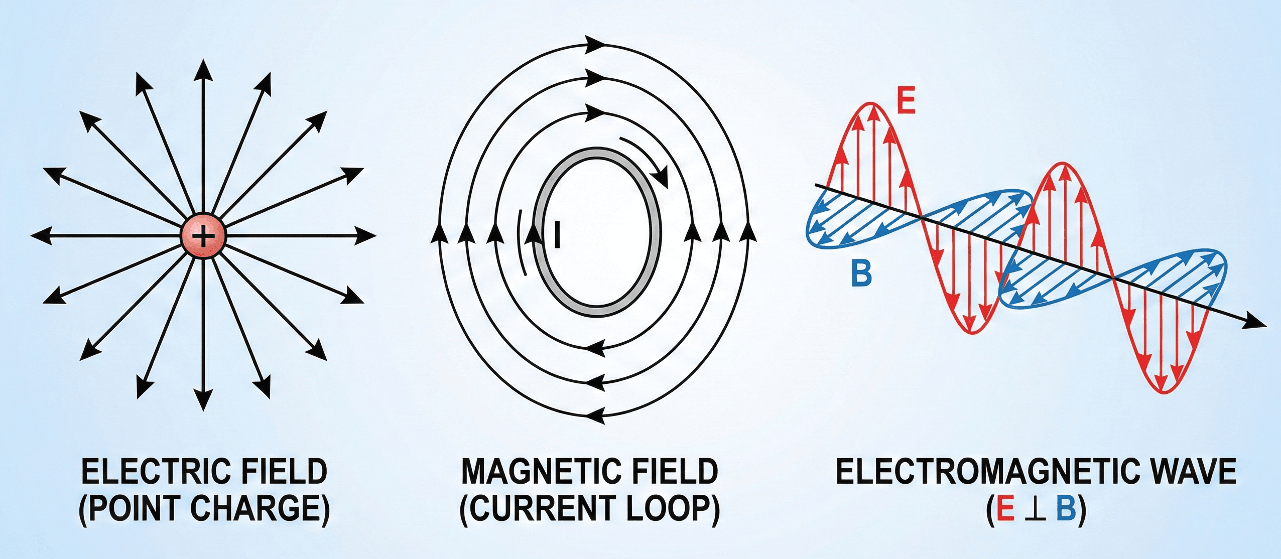
Electric and magnetic fields linked by charge, current, and changing fields
Maxwell’s Equation describes how electric and magnetic fields are created by charge, current, and changing electromagnetic fields.
The first thing to notice is that Maxwell’s Equation is not one isolated algebraic shortcut. It is a field framework that links electrostatics, magnetostatics, induction, and electromagnetic waves.
What is Maxwell’s Equation?
Maxwell’s Equation commonly refers to Maxwell’s equations, the four core equations of classical electromagnetism. Together, they describe how electric fields and magnetic fields behave in space and time.
In plain engineering language, Maxwell’s equations explain how charges create electric fields, why isolated magnetic poles are not part of ordinary electromagnetic theory, how changing magnetic fields induce electric fields, and how currents plus changing electric fields create magnetic fields.
These equations sit behind many simpler tools engineers use every day. Circuit equations such as Kirchhoff’s Voltage Law, device-level relationships such as capacitance and inductance, and wave concepts such as propagation and impedance all connect back to Maxwell’s field equations.
The Maxwell’s Equation formula
In differential form, the four Maxwell equations are commonly written as:
Each line answers a different physical question. Gauss’s law for electricity links electric field divergence to charge density. Gauss’s law for magnetism says magnetic field lines do not begin or end at isolated magnetic monopoles. Faraday’s law describes induction from changing magnetic fields. The Ampere-Maxwell law links magnetic curl to current and changing electric fields.
The same physics is often written in integral form when working with surfaces, loops, and flux:
In materials, engineers often use constitutive relationships to connect field intensity and flux density:
Pick the form based on the problem. Use differential form for local field behavior and simulation. Use integral form for symmetry, flux, loops, enclosed charge, and hand calculations.
Variables and units
Maxwell’s Equation uses field quantities rather than only lumped circuit quantities. That means the variables can change with position and time, especially in wave, antenna, motor, and high-frequency problems.
- \(\mathbf{E}\) Electric field intensity. SI units: volts per meter (V/m) or newtons per coulomb (N/C).
- \(\mathbf{B}\) Magnetic flux density. SI unit: tesla (T).
- \(\mathbf{D}\) Electric flux density. SI units: coulombs per square meter (C/m\(^2\)).
- \(\mathbf{H}\) Magnetic field intensity. SI units: amperes per meter (A/m).
- \(\rho\) Volume charge density. SI units: coulombs per cubic meter (C/m\(^3\)).
- \(\mathbf{J}\) Current density. SI units: amperes per square meter (A/m\(^2\)).
- \(\varepsilon\) Permittivity of a material. SI units: farads per meter (F/m). It affects electric-field behavior in dielectrics.
- \(\mu\) Permeability of a material. SI units: henries per meter (H/m). It affects magnetic-field behavior in materials.
Keep field quantities separate from lumped circuit quantities. Voltage is a potential difference, while electric field is voltage per distance. Current is total flow, while current density is current per area.
| Symbol | Meaning | SI units | Engineering interpretation |
|---|---|---|---|
| \(\mathbf{E}\) | Electric field | V/m | Force influence per unit charge or voltage gradient |
| \(\mathbf{B}\) | Magnetic flux density | T | Magnetic field effect used in motors, transformers, sensors, and inductors |
| \(\rho\) | Charge density | C/m\(^3\) | Source term for electric field divergence |
| \(\mathbf{J}\) | Current density | A/m\(^2\) | Distributed current flow through a conductor or region |
| \(\varepsilon\) | Permittivity | F/m | Controls electric-field response in dielectrics |
| \(\mu\) | Permeability | H/m | Controls magnetic-field response in magnetic materials |
If the physical size of a circuit is not small compared with the signal wavelength, field behavior and propagation delay can matter more than simple lumped-circuit intuition.
What each Maxwell equation means physically
A useful way to remember Maxwell’s Equation is to associate each line with the source or behavior it describes.
| Maxwell equation | Plain-language meaning | Engineering example |
|---|---|---|
| Gauss’s law for electricity | Electric charge creates electric flux. | Capacitors, insulation stress, electrostatic sensors, charged conductors |
| Gauss’s law for magnetism | Magnetic field lines form closed loops with no isolated magnetic source or sink. | Magnetic circuits, motors, transformers, magnetic shielding |
| Faraday’s law | A changing magnetic field induces an electric field. | Transformers, generators, inductors, induction heating, EMI pickup |
| Ampere-Maxwell law | Current and changing electric fields create magnetic fields. | Transmission lines, antennas, displacement current, high-frequency circuits |
When a problem feels confusing, identify the source first: charge, current, changing magnetic flux, or changing electric flux. That often tells you which Maxwell equation is doing the work.
Worked example: wave speed from Maxwell’s equations
Example problem
In free space, Maxwell’s equations predict electromagnetic waves that travel at speed \(c\). Use the free-space permittivity and permeability relationship to calculate the wave speed.
The wave-speed relationship is:
Substitute the standard free-space constants:
The result is approximately:
This is the speed of electromagnetic waves in free space. In materials, wave speed is reduced by permittivity and permeability, which is why dielectric materials affect propagation in cables, antennas, and transmission lines.
This example shows why Maxwell’s Equation is more than a static field tool. The equations predict traveling electromagnetic waves when electric and magnetic fields change with time.
Where engineers use Maxwell’s Equation
Engineers often use simplified circuit equations day to day, but Maxwell’s Equation is the deeper model behind many electrical and electromagnetic design decisions.
- Antennas and communications: predicting radiation, polarization, propagation, near fields, and far fields.
- Motors and generators: connecting current, magnetic fields, induced voltage, torque, and energy conversion.
- Transformers and inductors: understanding magnetic flux, induction, core materials, leakage, and saturation.
- Capacitors and insulation: evaluating electric fields, dielectric stress, stored energy, and breakdown risk.
- EMI and shielding: diagnosing field coupling, grounding issues, enclosure behavior, and cable emissions.
- High-speed circuits: understanding when traces behave as transmission lines instead of ideal wires.
Use lumped circuit laws when the geometry is electrically small and fields are contained well enough for voltage and current models. Move toward Maxwell-based field analysis when geometry, wavelength, boundary conditions, material properties, or radiation dominate behavior.
Assumptions and limitations
Maxwell’s equations are fundamental, but practical engineering use still depends on modeling assumptions. The challenge is usually not whether Maxwell’s equations are valid; it is whether the simplified form, material model, or boundary condition matches the real system.
- 1 The material properties \(\varepsilon\), \(\mu\), and conductivity are known or reasonably approximated.
- 2 Boundary conditions at conductors, dielectrics, magnetic materials, and interfaces are defined correctly.
- 3 The chosen approximation matches the frequency range, geometry, and wavelength of the problem.
- 4 Nonlinear, anisotropic, dispersive, or lossy materials are included when they affect the result.
Where simplified forms break down
Simple electrostatic, magnetostatic, or lumped-circuit models become less reliable when fields change quickly, wavelengths are comparable to geometry, materials are nonlinear, radiation is significant, or coupling between conductors cannot be ignored.
Do not use low-frequency circuit intuition alone for antennas, RF layouts, switching power converters, EMC problems, fast digital edges, or long transmission lines. Field effects may control the answer.
Engineering judgment and field reality
Maxwell’s Equation is exact within classical electromagnetism, but field modeling is only as good as the geometry, mesh, material data, boundary conditions, and frequency assumptions used to apply it.
Many real electromagnetic failures are layout problems, not equation problems. A fast switching loop, poor return path, sharp conductor edge, shield gap, or unexpected cable route can create fields the ideal schematic does not show.
When signal rise time, conductor length, or frequency makes the physical layout electrically large, stop thinking only in terms of ideal wires and start thinking in terms of fields, return paths, and propagation.
Common mistakes and engineering checks
- Treating Maxwell’s Equation as one formula: it is a set of coupled field equations, not a single plug-and-chug calculation.
- Mixing field and circuit quantities: voltage, current, electric field, magnetic flux density, and current density are related but not interchangeable.
- Ignoring boundary conditions: conductor surfaces, dielectric interfaces, and magnetic materials strongly shape the field solution.
- Using static assumptions at high frequency: time-varying fields create wave, radiation, and propagation effects.
- Assuming material constants are always constant: permittivity, permeability, and conductivity may vary with frequency, temperature, field strength, or direction.
Before trusting a field solution, check units, boundary conditions, material properties, mesh quality if simulated, and whether the result agrees with a simpler limiting case.
| Check item | What to verify | Why it matters |
|---|---|---|
| Field units | Separate V, A, V/m, T, A/m, and A/m\(^2\) | Prevents mixing lumped and distributed quantities |
| Boundary conditions | Define conductor, dielectric, magnetic, and open boundaries | Boundary conditions can dominate the solution |
| Frequency range | Check whether the problem is static, quasi-static, or wave-like | Determines whether propagation and radiation matter |
| Material model | Confirm \(\varepsilon\), \(\mu\), and conductivity assumptions | Materials control field strength, loss, speed, and coupling |
Frequently asked questions
Maxwell’s Equation usually refers to Maxwell’s equations, the four field equations that describe how electric and magnetic fields are produced, coupled, and propagated.
The four Maxwell equations are Gauss’s law for electricity, Gauss’s law for magnetism, Faraday’s law of induction, and the Ampere-Maxwell law.
Common SI quantities include electric field in V/m, magnetic flux density in tesla, charge density in C/m\(^3\), and current density in A/m\(^2\).
Advanced modeling is needed when geometry, materials, high frequency, wave propagation, radiation, boundary conditions, or coupling effects make simple circuit assumptions inaccurate.
Summary and next steps
Maxwell’s Equation is the foundation of classical electromagnetism. It connects electric fields, magnetic fields, charge, current, induction, and electromagnetic wave behavior.
The most important engineering judgment is choosing the right level of model. For low-frequency, electrically small circuits, lumped circuit laws may be enough. For antennas, RF systems, high-speed layouts, shielding, motors, transformers, and EMI problems, Maxwell-based field thinking becomes essential.
Where to go next
Continue your learning path with these curated next steps.
-
Prerequisite: Coulomb’s Law
Build electrostatic intuition for charge, electric force, and electric-field behavior.
-
Current topic: Maxwell’s Equation
Use this page as your reference for the four Maxwell equations, variables, assumptions, and engineering checks.
-
Advanced: Wave Propagation
Move from field equations into electromagnetic waves, propagation speed, antennas, and communications behavior.