Heat Transfer Calculator
Calculate heat transfer rate, heat flux, temperature difference, area, thickness, conductivity, convection coefficient, emissivity, U-value, or thermal resistance.
Calculator is for informational purposes only. Terms and Conditions
Choose what to solve for
Select the heat transfer method, unknown variable, and unit setup.
Enter the known values
Only the fields needed for the selected method and solve mode are shown.
Visual Check
Use the diagram to confirm the heat flow direction and active heat transfer method.
Solution
Live result, quick checks, warnings, and full solution steps.
Quick checks
- Heat flux—
Show solution steps See the equation, substitutions, assumptions, and result path
- Enter values to see the full solution steps and checks.
Source, Standards, and Assumptions
Calculation basis, constants, assumptions, and limitations.
Source/standard information updates based on the selected heat transfer method.
- Assumptions will appear after a valid calculation.
On this page
Calculator Guide
How to Use the Heat Transfer Calculator
The Heat Transfer Calculator above estimates heat transfer rate, heat flux, temperature difference, area, thermal conductivity, convection coefficient, emissivity, U-value, or total thermal resistance. Use it for conduction through solids, convection between a surface and fluid, radiation to surroundings, and simplified overall heat transfer through walls or assemblies.
The main goal is to choose the heat transfer mode that matches the physical situation. A solid wall usually uses conduction, a surface exposed to air or water usually uses convection, a hot surface radiating to surroundings uses radiation, and a full wall or layered assembly often uses U-value or total thermal resistance.
Quick Answer
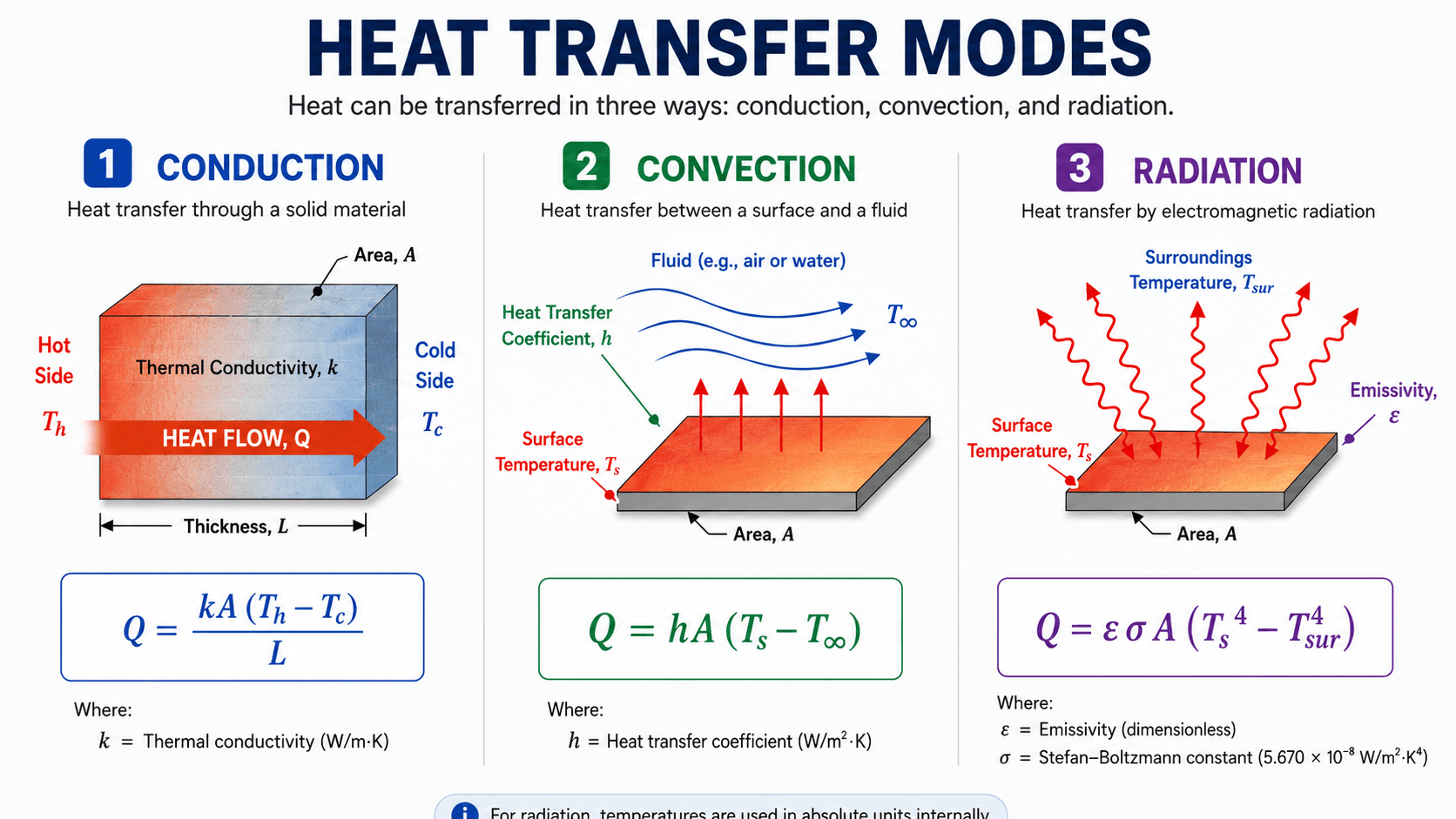
Heat transfer rate is the amount of heat energy moved per unit time. For a flat solid layer, use \(Q=kA\Delta T/L\). For convection, use \(Q=hA\Delta T\). For radiation, use \(Q=\varepsilon\sigma A(T_s^4-T_{sur}^4)\). For a full assembly with a known U-value, use \(Q=UA\Delta T\).
Do not rely on a simplified calculator when…
Do not use a simplified heat transfer result as the only basis for final equipment sizing, code compliance, fire-rated assemblies, pressure equipment, thermal stress design, heat exchanger design, or safety-critical insulation. Final design should verify geometry, material data, surface conditions, transient effects, radiation view factors, fluid properties, and project requirements.
Which Heat Transfer Method Should You Choose?
The most common user mistake is choosing the wrong heat transfer equation. Start with the physical situation, then select the matching calculator mode.
| Your Situation | Use This Calculator Mode | Main Formula |
|---|---|---|
| Heat through a wall, slab, plate, insulation layer, or solid material | Conduction | \(Q=kA\Delta T/L\) |
| Heat from a surface to air, water, oil, steam, or another fluid | Convection | \(Q=hA\Delta T\) |
| Heat emitted from a hot surface to cooler surroundings | Radiation | \(Q=\varepsilon\sigma A(T_s^4-T_{sur}^4)\) |
| Heat loss through a full wall, window, roof, assembly, or simplified heat exchanger surface | Overall U-value | \(Q=UA\Delta T\) |
| You already know the total thermal resistance in \(K/W\) | Total resistance | \(Q=\Delta T/R_{total}\) |
Inputs and Outputs Used by the Calculator
The calculator changes the required inputs based on the selected method and solve mode. Most heat transfer problems need an area, temperature difference, and one property that controls how easily heat moves.
| Type | Value | What It Means | Common Unit |
|---|---|---|---|
| Input | Temperature Difference, \(\Delta T\) | Driving force for heat transfer between hot and cold regions. | K, °C, °F |
| Input | Area, \(A\) | Surface or cross-sectional area available for heat transfer. | m², ft² |
| Input | Thermal Conductivity, \(k\) | Material property used for conduction through solids. | W/m·K |
| Input | Thickness, \(L\) | Conduction path length through the solid layer. | m, mm, in, ft |
| Input | Convection Coefficient, \(h\) | Surface-to-fluid heat transfer coefficient. | W/m²·K |
| Input | Emissivity, \(\varepsilon\) | Surface radiation effectiveness from 0 to 1. | dimensionless |
| Input | U-Value, \(U\) | Overall heat transfer coefficient for a full assembly or system. | W/m²·K |
| Input | Total Resistance, \(R_{total}\) | Absolute resistance for the full heat flow path. | K/W |
| Output | Heat Transfer Rate, \(Q\) | Total thermal energy transferred per unit time. | W, kW, BTU/hr |
| Output | Heat Flux, \(q”\) | Heat transfer rate per unit area. | W/m², BTU/hr·ft² |
Heat Transfer Formulas Used
Heat transfer is calculated with different formulas depending on the physical mechanism. The calculator uses conduction, convection, radiation, U-value, and total resistance relationships.
Conduction Through a Flat Solid
Use this for steady heat transfer through a wall, slab, plate, insulation layer, or other solid material.
Convection From a Surface
Use this when heat is transferred between a solid surface and a surrounding fluid such as air or water.
Radiation to Surroundings
Radiation must use absolute temperature. The calculator converts °C and °F to absolute temperature internally before applying the fourth-power relationship.
Overall U-Value Method
Use this when an overall heat transfer coefficient is known for a wall, assembly, heat exchanger surface, or simplified thermal system.
Total Thermal Resistance Method
Use this when the total absolute thermal resistance is already known in \(K/W\) or equivalent units.
Important: \(R_{total}\), R-value, and U-value are not always the same type of resistance
Do not mix absolute thermal resistance with area-normalized R-value. The calculator’s total resistance mode uses absolute resistance \(R_{total}\) in \(K/W\), so \(Q=\Delta T/R_{total}\). Building-envelope U-values usually use area-normalized resistance \(R”_{total}\) in \(m^2K/W\), where \(U=1/R”_{total}\) and \(Q=UA\Delta T\).
Radiation temperature warning
For radiation, \(100°C\) and \(20°C\) must be converted to \(373.15K\) and \(293.15K\). Do not calculate \(100^4-20^4\). The physically correct radiation term uses \(373.15^4-293.15^4\).
What the Variables Mean
Every symbol in a heat transfer calculation must match the selected method. Using a conduction property in a convection formula, or using Celsius directly in a radiation fourth-power term, will produce an unreliable result.
| Symbol | Meaning | How to Enter It |
|---|---|---|
| \(Q\) | Heat transfer rate. | Enter or read as W, kW, BTU/hr, or another heat-rate unit. |
| \(q”\) | Heat flux, or heat transfer per unit area. | Calculated from \(q”=Q/A\) when area is known. |
| \(k\) | Thermal conductivity of a solid material. | Use a material value in W/m·K or BTU/hr·ft·°F. |
| \(A\) | Heat transfer area. | Use the surface or cross-sectional area normal to the heat flow path. |
| \(L\) | Thickness or conduction path length. | Use the distance heat travels through the solid. |
| \(h\) | Convective heat transfer coefficient. | Use a coefficient appropriate for fluid, flow condition, and surface geometry. |
| \(\varepsilon\) | Emissivity of the surface. | Enter a dimensionless value greater than 0 and less than or equal to 1. |
| \(\sigma\) | Stefan-Boltzmann constant. | \(\sigma=5.670374419\times10^{-8}\,W/(m^2K^4)\). |
| \(U\) | Overall heat transfer coefficient. | Use when all layer and surface effects are combined into one coefficient. |
| \(R_{total}\) | Absolute total thermal resistance. | Use \(K/W\) when calculating \(Q=\Delta T/R_{total}\). |
| \(R”_{total}\) | Area-normalized total resistance. | Use \(m^2K/W\) when calculating \(U=1/R”_{total}\). |
How to Use the Calculator
Start by matching the calculation method to the physical heat transfer situation. Then choose the unknown value, enter the known inputs, select units, and review the result with the quick checks.
Choose the heat transfer method
Use conduction for solids, convection for surface-to-fluid transfer, radiation for emitted thermal radiation, and U-value or resistance for full assemblies.
Select the solve mode
Choose whether to solve for heat transfer rate, temperature, area, thickness, conductivity, convection coefficient, emissivity, U-value, or resistance.
Check unit selectors
Make sure temperature units, length units, area units, and material-property units match the values you are entering.
Review heat flux and direction
After calculating \(Q\), also review heat flux, temperature difference, and whether the sign indicates heat flow in the expected direction.
How to Interpret Heat Transfer Results
A heat transfer result is most useful when you understand both the total heat rate and the heat flux. Heat rate tells you the total load, while heat flux tells you how intense that load is over the surface.
| Result Pattern | What It May Mean | What to Check Next |
|---|---|---|
| \(Q=0\) | No net heat transfer because the temperature difference is zero. | Confirm the hot and cold temperatures are not accidentally equal. |
| Positive \(Q\) | Heat flows in the labeled hot-to-cold direction. | Check whether that direction matches the physical system. |
| Negative \(Q\) | The actual heat flow is opposite the assumed direction. | Verify which side is hotter and whether temperature signs are correct. |
| Very high heat flux | Large heat load concentrated over a small area. | Check area, material data, and whether the simplified model is appropriate. |
| Unrealistic solved property | The inputs may be inconsistent or the selected method may be wrong. | Check units, temperatures, and whether conduction, convection, radiation, or U-value is the correct model. |
What to do with the result
Use heat transfer rate \(Q\) to estimate total heating or cooling load, equipment load, insulation loss, or energy transfer. Use heat flux \(q”\) to compare surface intensity, material limits, thermal comfort, or whether a heat sink, wall, insulation layer, or surface area is large enough.
What changes the result most?
Temperature difference and area often dominate simple heat transfer calculations because \(Q\) scales directly with both. For conduction, thickness and conductivity are equally important because doubling thickness cuts \(Q\) in half, while doubling conductivity doubles \(Q\). For radiation, absolute temperature dominates because temperature is raised to the fourth power.
Heat Transfer Rate vs Heat Flux
Heat transfer rate and heat flux are related, but they answer different engineering questions. Heat transfer rate tells you the total heat flow, while heat flux tells you how concentrated that heat flow is over a surface.
Heat Flux Formula
\(Q\) answers “how much total heat is transferred?” while \(q”\) answers “how intense is heat transfer per unit surface area?”
Input Quality Checklist
Heat transfer formulas are simple, but the result can be wrong if the inputs do not describe the same physical system. Check these items before trusting the output.
Correct Method
Verify that the selected method matches the situation: solid conduction, surface convection, radiation, U-value, or total resistance.
Temperature Difference
Confirm which side is hot and which side is cold. For radiation, use absolute temperature internally.
Area Definition
Use the heat-transfer area, not room floor area or material volume unless that is truly the exposed transfer surface.
Material Property
Use a realistic conductivity, convection coefficient, emissivity, or U-value for the actual surface and operating condition.
Layer Thickness
For conduction, use thickness in the heat flow direction. A unit error between inches and meters can create a huge error.
Steady-State Assumption
Simple heat transfer formulas assume conditions are not changing quickly with time.
Step-by-Step Worked Examples
Worked examples help verify that the calculator result is reasonable. These examples show conduction through a flat wall, U-value heat loss, and the radiation temperature conversion users most often miss.
Formula
Substitute Values
Calculate
Result
Heat transfer rate: \(800\,W\), or \(0.8\,kW\). The heat flux is \(q”=800/10=80\,W/m^2\).
Formula
Substitute Values
Calculate
Result
Wall heat loss: \(175\,W\). This is the simplified heat transfer rate through the full assembly using the known U-value.
Example 3: Radiation temperature conversion
If a surface is \(100°C\) and the surroundings are \(20°C\), the radiation formula should use \(373.15K\) and \(293.15K\), not 100 and 20. For \(\varepsilon=0.9\) and \(A=1m^2\), the radiation equation is approximately:
Thermal Resistance and U-Value Diagram
Wall heat loss often depends on the resistance of several layers. The diagram below shows how indoor air, surface films, material layers, and outdoor air combine into a total resistance path.
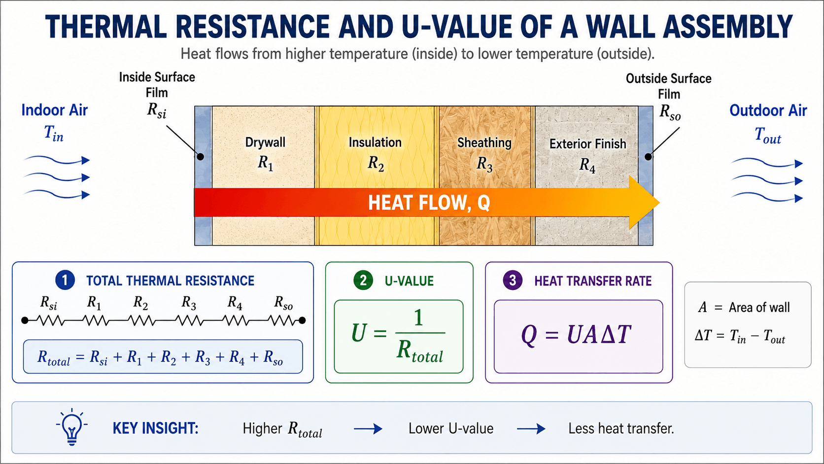
Use the right resistance type
A full wall assembly commonly uses area-normalized resistance \(R”_{total}\), where \(U=1/R”_{total}\). The calculator’s total resistance mode uses absolute resistance \(R_{total}\) in \(K/W\), where \(Q=\Delta T/R_{total}\).
Typical Reference Values
Reference values vary by material, temperature, surface condition, fluid velocity, and geometry. These are approximate room-temperature reference ranges. Use manufacturer data, test data, or project-specific values for final calculations.
| Category | Quantity | Typical Range or Example | Use With |
|---|---|---|---|
| Insulation | Fiberglass insulation conductivity | About \(0.03\) to \(0.05\,W/(m\cdot K)\) | Conduction |
| Building material | Wood conductivity | About \(0.10\) to \(0.20\,W/(m\cdot K)\) | Conduction |
| Building material | Concrete conductivity | Often about \(1\) to \(2\,W/(m\cdot K)\) | Conduction |
| Metal | Steel conductivity | Often tens of \(W/(m\cdot K)\) | Conduction |
| Fluid surface | Natural convection in air | Often about \(5\) to \(25\,W/(m^2K)\) | Convection |
| Fluid surface | Forced convection in air | Often about \(25\) to \(250\,W/(m^2K)\) | Convection |
| Fluid surface | Water convection | Can be hundreds to thousands of \(W/(m^2K)\) | Convection |
| Surface radiation | Painted or dark surface emissivity | Often \(0.8\) to \(0.95\) | Radiation |
| Surface radiation | Polished metal emissivity | Often much lower, sometimes below \(0.1\) | Radiation |
Practical insight
Low thermal conductivity materials reduce conduction, but radiation and convection at the surfaces can still matter. A well-insulated assembly may be limited by surface film resistance, thermal bridging, or air leakage rather than only material conductivity.
Design Ranges and Practical Judgment
A mathematically valid heat transfer result is not always a design-ready answer. Real systems may include multiple layers, changing temperatures, surface films, air gaps, contact resistance, radiation view factors, thermal bridges, and nonuniform flow.
Low Heat Transfer
Low \(Q\) may indicate good insulation, small area, small temperature difference, or high resistance.
Moderate Heat Transfer
A moderate result may be reasonable for building walls, insulated components, and steady heating or cooling estimates.
High Heat Transfer
High \(Q\) or high heat flux may indicate thin material, large area, high temperature difference, high \(h\), or high \(U\).
Engineering judgment check
If the calculation is for equipment protection, burns, heat sinks, insulation thickness, building envelope performance, or energy use, verify the simplified result with project-specific data. The right value of \(h\), \(U\), or \(\varepsilon\) often matters more than extra decimal places in the calculator result.
Heat Transfer Units and Conversions
Unit consistency is one of the most important parts of heat transfer calculations. The calculator can convert units, but the entered values must still represent the correct physical quantity.
| Quantity | Common Units | Conversion Reminder |
|---|---|---|
| Heat transfer rate | W, kW, BTU/hr, kcal/hr | \(1\,kW=1000\,W\); \(1\,BTU/hr\approx0.293\,W\) |
| Area | m², cm², ft², in² | \(1\,ft^2\approx0.0929\,m^2\) |
| Length or thickness | m, cm, mm, in, ft | \(1\,in=0.0254\,m\) |
| Thermal conductivity | W/m·K, BTU/hr·ft·°F | Use a value that matches the material and unit system. |
| Convection or U-value | W/m²·K, BTU/hr·ft²·°F | These are area-based heat transfer coefficients. |
| Absolute thermal resistance | K/W, hr·°F/BTU | \(1\,hr\cdot°F/BTU\approx1.8956\,K/W\) |
| Area-normalized R-value | m²K/W, hr·ft²·°F/BTU | Use area-normalized resistance when relating \(U=1/R”\). |
| Temperature | °C, °F, K, °R | Radiation uses absolute temperature; \(\Delta T\) in °C equals \(\Delta T\) in K. |
Conduction vs. Convection vs. Radiation vs. U-Value
The best method depends on the dominant heat transfer path. Many real systems include more than one mode, but simplified calculations usually isolate the most important mechanism.
| Method | Best For | Main Inputs | Main Caution |
|---|---|---|---|
| Conduction | Heat through solids, walls, slabs, insulation, and plates. | \(k\), \(A\), \(L\), \(\Delta T\) | Assumes steady, one-dimensional heat flow through a flat layer. |
| Convection | Heat between a surface and air, water, or another fluid. | \(h\), \(A\), \(\Delta T\) | The value of \(h\) can vary widely with flow and geometry. |
| Radiation | Thermal emission from a surface to surroundings. | \(\varepsilon\), \(A\), absolute temperatures | Temperature must be absolute and view factors may matter in real systems. |
| U-Value | Full assemblies, walls, windows, and simplified system heat loss. | \(U\), \(A\), \(\Delta T\) | Requires a valid overall coefficient for the complete heat path. |
| Total Resistance | Layered systems where total absolute resistance is known. | \(R_{total}\), \(\Delta T\) | All relevant layer and surface resistances must be included correctly. |
Common Mistakes That Cause Wrong Results
Most heat transfer errors come from choosing the wrong method, using the wrong area, or mixing unit systems.
Common Mistakes
- Using Celsius directly in the radiation fourth-power formula.
- Entering wall floor area instead of heat-transfer surface area.
- Using material conductivity \(k\) when an overall U-value is needed.
- Mixing absolute \(K/W\) resistance with area-normalized \(m^2K/W\) R-value.
- Forgetting that thicker insulation lowers conduction heat transfer.
- Using a generic convection coefficient without checking the flow condition.
- Ignoring surface film resistance in wall or assembly heat loss.
Better Practice
- Choose the heat transfer mode before entering values.
- Use absolute temperature for radiation calculations.
- Use the area normal to the heat flow direction.
- Check whether the problem needs \(k\), \(h\), \(U\), or \(R_{total}\).
- Verify unit selectors whenever switching between SI and U.S. units.
- Compare heat flux, not just total heat transfer rate.
Troubleshooting Unexpected Results
If the calculator result looks unreasonable, check the method, units, and physical direction of heat flow before changing formulas.
| Problem | Likely Cause | Fix |
|---|---|---|
| Result is negative | The cold side may be hotter than the hot side based on entered values. | Check temperature order and whether negative heat flow is meaningful for your sign convention. |
| Heat transfer is far too large | Area too large, thickness too small, units wrong, or coefficient too high. | Check m² vs ft², mm vs m, and W vs kW. |
| Radiation result seems impossible | Temperature was treated incorrectly or emissivity is unrealistic. | Use absolute temperature and verify \(\varepsilon\) is between 0 and 1. |
| U-value result does not match conduction result | U-value includes surface and layer effects while simple conduction may include only one layer. | Compare the complete heat path and confirm which resistances are included. |
| Zero heat transfer | Temperature difference is zero. | Check whether the same temperature was entered on both sides by mistake. |
| Emissivity above 1 | The heat rate, area, or radiation temperatures are inconsistent. | Emissivity must be greater than 0 and less than or equal to 1. |
| Negative area, thickness, U-value, or conductivity | The selected solve mode and signs are physically inconsistent. | Check temperature direction, heat flow sign, and selected method. |
Common edge case
A result can be mathematically valid but practically misleading when temperature, material properties, or flow conditions change over time. In those cases, a transient heat transfer model or detailed thermal simulation may be more appropriate.
Field Measurement Notes
Heat transfer calculations are only as good as the measured inputs. These practical notes help prevent common field-data mistakes.
IR Thermometer Emissivity
Infrared temperature readings depend on emissivity settings. Shiny metals can read incorrectly if emissivity is not adjusted.
Surface vs Air Temperature
Air temperature near a surface may not equal the bulk room or outdoor temperature, especially near vents, windows, or heated equipment.
Installed Thickness
Use actual installed insulation thickness, not nominal thickness, especially if insulation is compressed or uneven.
Moisture Effects
Wet insulation can have a much higher effective thermal conductivity than dry insulation.
Thermal Bridging
Metal studs, fasteners, frames, and structural members can bypass insulation and increase heat loss.
Air Leakage
Air leaks can dominate real building heat loss even when the conductive wall calculation looks low.
Assumptions, Sources, and Limitations
This calculator is intended for educational use, preliminary estimates, and quick engineering checks. It uses standard steady-state heat transfer relationships and assumes the input properties represent the actual operating condition.
Steady-State Assumption
The formulas assume temperatures and properties are not changing rapidly with time.
Geometry Assumption
Flat-wall conduction assumes one-dimensional heat flow through a uniform thickness.
Property Assumption
Material properties, convection coefficients, U-values, and emissivity are treated as constant inputs.
Design Limitation
The calculator does not perform code review, CFD, transient modeling, detailed heat exchanger design, or thermal stress analysis.
Calculation basis
The formulas used here are standard heat transfer relationships: Fourier-style conduction through a flat layer, Newton’s law of cooling for convection, the Stefan-Boltzmann radiation relationship, the overall heat transfer relationship \(Q=UA\Delta T\), and the resistance relationship \(Q=\Delta T/R_{total}\). For additional reference on standard engineering heat transfer relationships and overall heat transfer coefficients, see Engineering ToolBox: Overall Heat Transfer Coefficient.
Glossary of Heat Transfer Terms
These definitions help explain the calculator inputs and outputs in plain engineering language.
Heat Transfer Rate
The total amount of heat energy transferred per unit time, usually measured in watts or BTU/hr.
Heat Flux
Heat transfer rate divided by area. It shows how intense the heat transfer is at a surface.
Thermal Conductivity
A material property that describes how easily heat conducts through a solid.
Convection Coefficient
A coefficient that describes heat transfer between a surface and a fluid.
Emissivity
A dimensionless surface property that describes how effectively a surface emits thermal radiation.
U-Value
The overall heat transfer coefficient for a full assembly, including layers and surface effects.
Absolute Thermal Resistance
A resistance in \(K/W\) used directly with \(Q=\Delta T/R_{total}\).
Area-Normalized R-Value
A resistance in \(m^2K/W\) used with \(U=1/R”_{total}\) for building assemblies.
Temperature Difference
The difference between the hot and cold sides. It is the main driving force for heat transfer.
Frequently Asked Questions
What does a heat transfer calculator calculate?
A heat transfer calculator estimates heat transfer rate, heat flux, temperature difference, area, conductivity, convection coefficient, emissivity, U-value, or total thermal resistance depending on the selected method and solve mode.
What formula is used for heat transfer?
Common heat transfer formulas include \(Q=kA\Delta T/L\) for conduction, \(Q=hA\Delta T\) for convection, \(Q=\varepsilon\sigma A(T_s^4-T_{sur}^4)\) for radiation, \(Q=UA\Delta T\) for overall heat transfer, and \(Q=\Delta T/R_{total}\) for thermal resistance.
Why does radiation heat transfer use Kelvin?
Radiation heat transfer uses absolute temperature because the Stefan-Boltzmann equation depends on the fourth power of absolute temperature. Celsius and Fahrenheit must be converted to Kelvin or Rankine before using the radiation formula.
What is the difference between heat transfer rate and heat flux?
Heat transfer rate is the total heat flow, usually in watts or BTU per hour. Heat flux is heat transfer rate divided by area, usually in \(W/m^2\) or \(BTU/hr\cdot ft^2\).
Can heat transfer be negative?
Yes. A negative heat transfer rate usually means heat is flowing opposite the assumed direction. It often happens when the entered cold-side temperature is actually higher than the hot-side temperature.
Can this calculator be used for final thermal design?
The calculator is useful for estimates, learning, and early engineering checks, but final design should verify geometry, material data, temperature-dependent properties, boundary conditions, safety factors, and applicable project requirements.