Key Takeaways
- Definition: Specific heat capacity tells you how much heat energy is needed to raise a material’s temperature by a given amount.
- Main use: Engineers use \(Q = mc\Delta T\) to estimate heating or cooling energy for solids, liquids, gases, and thermal systems.
- Watch for: The simple equation assumes no phase change, reasonably uniform temperature, known mass, and a suitable value of \(c\).
- Outcome: You will be able to solve for heat energy, mass, specific heat capacity, or temperature change while checking units and assumptions.
Table of Contents
Heat energy, mass, and temperature change in a material
The specific heat capacity equation relates heat energy, mass, specific heat, and temperature change for a material.
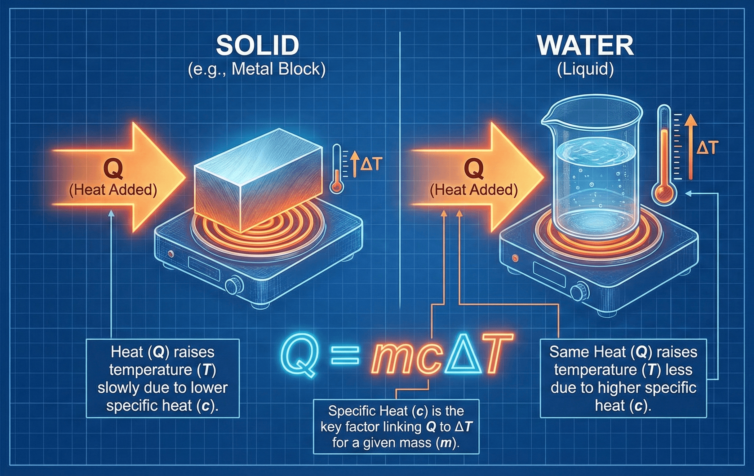
The first thing to notice is that temperature change is not determined by heat input alone. The same heat input can create a small temperature rise in a large mass or a large temperature rise in a small mass, depending on the material’s specific heat capacity.
What is the specific heat capacity equation?
The specific heat capacity equation estimates the heat energy required to change the temperature of a substance without changing its phase. In engineering terms, it answers a common design question: how much energy must be added or removed to heat or cool a known amount of material?
Specific heat capacity, usually written as \(c\), is a material property. A material with a high specific heat capacity needs more energy for the same temperature rise. Water is a common example: it takes much more energy to heat water than the same mass of many metals by the same temperature difference.
This equation is used in heat-transfer calculations, thermal storage estimates, equipment warm-up and cooldown checks, HVAC loads, laboratory calorimetry, process heating, electronics thermal design, and basic thermodynamics problems.
The specific heat capacity formula
The most common engineering form of the specific heat capacity equation is:
This equation says that heat energy \(Q\) increases in direct proportion to mass \(m\), specific heat capacity \(c\), and temperature change \(\Delta T\). If any one of those three terms doubles while the others stay the same, the required heat energy doubles.
Temperature change is usually written as:
Use a temperature difference, not just a final temperature. A change of \(1\,\text{K}\) is equal in size to a change of \(1^\circ\text{C}\), so Celsius differences and kelvin differences are numerically interchangeable for \(\Delta T\).
Confirm whether the problem is asking for heat energy, heat rate, or temperature rise. \(Q = mc\Delta T\) gives energy, not power, unless it is divided by time.
Variables and units
The equation is simple, but unit consistency matters. The most common mistake is mixing joules, kilojoules, grams, kilograms, Celsius, and kelvin without converting the specific heat capacity value to match.
- \(Q\) Heat energy added or removed. Common SI units are joules (J) or kilojoules (kJ). US customary units often use BTU.
- \(m\) Mass of the material being heated or cooled. Common SI units are kilograms (kg) or grams (g).
- \(c\) Specific heat capacity of the material. Common SI units are J/(kg·K), kJ/(kg·K), or J/(g·°C).
- \(\Delta T\) Temperature change, calculated as final temperature minus initial temperature. Use K or °C difference consistently.
If \(c\) is in J/(kg·K), use mass in kg and temperature difference in K or °C difference. If \(c\) is in J/(g·°C), use mass in grams.
| Variable | Meaning | SI units | US customary units | Engineering note |
|---|---|---|---|---|
| \(Q\) | Heat energy | J, kJ | BTU | Positive when heat is added, negative when heat is removed if using a sign convention. |
| \(m\) | Mass | kg, g | lbm | Use mass, not volume, unless density is used to convert volume to mass. |
| \(c\) | Specific heat capacity | J/(kg·K) | BTU/(lbm·°F) | Depends on material and may vary with temperature. |
| \(\Delta T\) | Temperature change | K or °C difference | °F difference | Use a temperature difference, not an absolute temperature value. |
Water has a high specific heat capacity, about \(4.18\,\text{kJ/(kg·K)}\). Heating \(1\,\text{kg}\) of water by \(10^\circ\text{C}\) takes about \(41.8\,\text{kJ}\).
How to rearrange the specific heat capacity equation
The same equation can solve for heat energy, mass, specific heat capacity, or temperature change. The best form depends on what the problem gives you and what you are trying to find.
After rearranging, check the units of the answer. For example, \(Q/(m\Delta T)\) should reduce to energy per mass per temperature difference, which is the unit of specific heat capacity.
Worked example: heating water
Example problem
Estimate the heat energy required to raise \(2.5\,\text{kg}\) of water from \(20^\circ\text{C}\) to \(75^\circ\text{C}\). Use \(c = 4.18\,\text{kJ/(kg·K)}\).
First calculate the temperature change:
Substitute the known values into the specific heat capacity equation:
The kg and K units cancel, leaving heat energy in kJ:
This is the ideal heat absorbed by the water. A real heater may require more input energy because heat is also lost to the container, surrounding air, piping, or equipment surfaces.
Where engineers use this equation
The specific heat capacity equation appears anywhere engineers need to estimate sensible heating or cooling. “Sensible” means the temperature changes, but the material does not melt, freeze, boil, condense, or chemically react during the calculation.
- Thermal storage: estimating how much energy a tank, battery pack, concrete slab, or water volume can absorb.
- HVAC and process heating: estimating heating or cooling loads for fluids, tanks, coils, and controlled spaces.
- Manufacturing: calculating preheat energy for metals, plastics, ceramics, and process materials.
- Electronics cooling: estimating transient temperature rise in components before steady heat-transfer paths dominate.
- Laboratory calorimetry: determining unknown heat capacity or heat exchange from measured temperature changes.
Use \(Q = mc\Delta T\) when the main result is sensible energy storage or temperature change. Use Fourier’s Law when the main result is heat-transfer rate through a material. Use latent heat relationships when phase change occurs.
Assumptions and limitations
The specific heat capacity equation is reliable when the material can be treated as a single substance with a known average heat capacity over the temperature range of interest.
- 1 No phase change occurs during the temperature change.
- 2 The material is reasonably uniform, or an effective average \(c\) value is appropriate.
- 3 The temperature is sufficiently uniform, or the calculation is clearly an average bulk-temperature estimate.
- 4 Heat losses, container heating, and environmental exchange are either negligible or handled separately.
Neglected factors
The simple form does not account for heat loss to surroundings, temperature gradients inside the object, phase change, chemical reaction, evaporation, nonuniform mixing, or strong variation of \(c\) with temperature.
Do not use \(Q = mc\Delta T\) by itself across melting, freezing, boiling, or condensation. Phase changes require latent heat terms in addition to sensible heat.
Engineering judgment and field reality
In real systems, the equation often gives the ideal heat absorbed by the target material, not the total energy that must be supplied by equipment. Actual energy input may be higher because heaters, tanks, insulation, piping, air gaps, and surrounding structures also absorb or lose heat.
A tank-heating calculation may look correct on paper but underpredict warm-up time if it ignores heat loss through the tank wall, energy absorbed by the tank shell, mixing limitations, or stratification between hot and cold fluid layers.
If the real system includes a heater, vessel, piping, insulation, or airflow, treat \(mc\Delta T\) as the useful energy into the material and then add losses or efficiency separately.
Common mistakes and engineering checks
- Mixing grams and kilograms: using \(c\) in J/(kg·K) with mass in grams can create a 1,000× error.
- Using final temperature instead of temperature change: the equation uses \(\Delta T\), not \(T_f\) alone.
- Ignoring phase change: boiling, freezing, melting, or condensation requires latent heat.
- Confusing heat energy and heat rate: \(Q\) is energy; power requires dividing energy by time.
- Assuming constant \(c\) over a large temperature range: some materials need a temperature-dependent heat capacity model.
For SI calculations, multiply kg by kJ/(kg·K) by K. If the result is not in kJ, your units are probably mismatched.
| Check item | What to verify | Why it matters |
|---|---|---|
| Temperature difference | Use \(T_f – T_i\), not final temperature alone | The equation depends on change in temperature |
| Mass basis | Match kg with J/(kg·K) or g with J/(g·°C) | Prevents 1,000× conversion errors |
| Phase state | Confirm no melting, boiling, freezing, or condensation | Phase change requires latent heat |
| System boundary | Decide whether container, piping, or heat losses are included | Prevents underestimating real equipment energy input |
Frequently asked questions
The specific heat capacity equation is \(Q = mc\Delta T\). It calculates the heat energy needed to change the temperature of a known mass of material.
Common SI units are J/(kg·K), kJ/(kg·K), or J/(g·°C). US customary calculations often use BTU/(lbm·°F).
Rearrange \(Q = mc\Delta T\) depending on the unknown: \(c = Q/(m\Delta T)\), \(m = Q/(c\Delta T)\), or \(\Delta T = Q/(mc)\).
The simple form becomes less reliable when phase change occurs, heat losses are significant, temperature is not uniform, or the material’s specific heat changes strongly with temperature.
Summary and next steps
The specific heat capacity equation \(Q = mc\Delta T\) is the core relationship for sensible heating and cooling. It connects heat energy to mass, material heat capacity, and temperature change.
The main engineering judgment is knowing when the simple equation is enough. If no phase change occurs and heat losses are small or handled separately, it is a fast and useful estimate. If heat-transfer rate, insulation, conduction paths, or equipment losses matter, pair it with heat-transfer methods and real system assumptions.
Where to go next
Continue your learning path with these curated next steps.
-
Prerequisite: Heat Transfer
Build the broader foundation behind heat movement, thermal energy, conduction, convection, and radiation.
-
Current topic: Specific Heat Capacity Equation
Use this page as your reference for \(Q = mc\Delta T\), units, rearrangements, and common engineering checks.
-
Next step: Fourier’s Law
Move from stored thermal energy to heat-transfer rate through materials and temperature gradients.