Key Takeaways
- Definition: Kirchoff’s Voltage Law says the algebraic sum of voltage rises and drops around a closed circuit loop equals zero.
- Main use: Engineers use KVL to write loop equations, solve unknown voltages, check circuit consistency, and troubleshoot series or mesh circuits.
- Watch for: Most errors come from inconsistent sign convention, incorrect assumed current direction, or treating high-frequency circuits as ideal lumped circuits.
- Outcome: You will be able to write a KVL loop equation, solve an unknown voltage, and check whether your circuit result is physically reasonable.
Table of Contents
Voltage rises and voltage drops around a closed circuit loop
Kirchoff’s Voltage Law states that voltage rises and drops around any closed circuit loop must sum to zero.
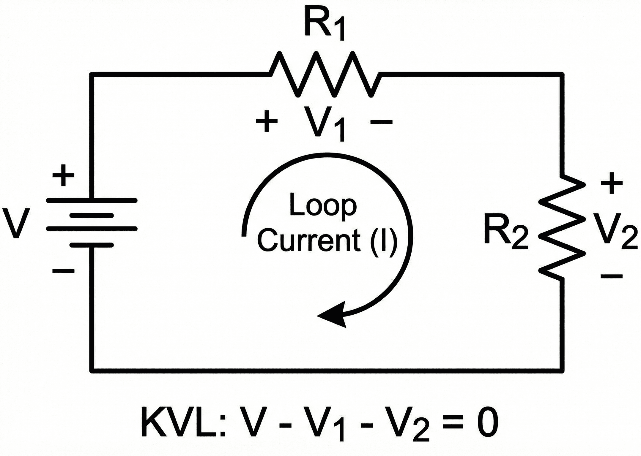
The first thing to notice is that KVL is a loop rule. You start at one point, move around a closed path, add each voltage rise or drop with a consistent sign convention, and return to the starting voltage.
What is Kirchoff’s Voltage Law?
Kirchoff’s Voltage Law, often abbreviated as KVL, is a circuit-analysis rule based on conservation of energy. It says that the total voltage gained and lost around a closed circuit loop must balance.
In practical terms, if a battery or power supply adds voltage to a loop, the resistors, loads, LEDs, motors, wires, or other components in that loop must account for that voltage through drops or rises. If the loop equation does not balance, the assumed voltages, polarities, current direction, or component values need to be checked.
The law is commonly spelled Kirchhoff’s Voltage Law in textbooks, but this page follows the keyword spelling Kirchoff’s Voltage Law while explaining the same KVL circuit principle.
The Kirchoff’s Voltage Law formula
The most compact form of Kirchoff’s Voltage Law is:
This means the algebraic sum of every voltage change around a closed loop equals zero. The word “algebraic” matters because each voltage must be assigned a sign based on your chosen loop direction and polarity convention.
A common series circuit form is:
Rearranged, the same loop says the source voltage equals the sum of the voltage drops:
If a resistor voltage is unknown and current is known, Ohm’s Law can be paired with KVL:
Pick one loop direction and one voltage sign convention before writing the equation. A negative answer is not automatically wrong; it often means the actual polarity is opposite your assumption.
Variables and units
KVL works with voltage changes around a closed path. The units are usually simple, but the sign convention is where most mistakes happen.
- \(\sum V\) Algebraic sum of voltage rises and drops around the loop. Unit: volts (V).
- \(V_s\) Source voltage supplied by a battery, power supply, generator, or equivalent source. Unit: volts (V).
- \(V_1, V_2, V_3\) Voltage drops or rises across individual circuit elements. Unit: volts (V).
- \(I\) Loop or branch current when Ohm’s Law is used with KVL. Unit: amperes (A).
- \(R\) Resistance of a component or equivalent resistance. Unit: ohms (\(\Omega\)).
Every term in a KVL loop equation must be a voltage. If you include \(IR\), it is valid because amperes times ohms equals volts.
| Quantity | Meaning | SI unit | Common source of error | Engineering note |
|---|---|---|---|---|
| \(V_s\) | Source voltage | V | Wrong polarity sign | Crossing from negative to positive terminal is usually a voltage rise. |
| \(V_R\) | Resistor voltage | V | Using current direction inconsistently | Passive sign convention usually treats current entering the positive side of a resistor. |
| \(I\) | Current | A | Assuming current direction incorrectly | A negative solved current means actual direction is opposite the assumed arrow. |
| \(R\) | Resistance | \(\Omega\) | Using k\(\Omega\) as \(\Omega\) | Convert \(1\,\text{k}\Omega = 1000\,\Omega\). |
In a single-loop DC resistor circuit, the source voltage should equal the sum of all resistor voltage drops. If the drops exceed the source, a current, resistance, or polarity assumption is wrong.
How to use KVL sign convention
Kirchoff’s Voltage Law is less about rearranging one formula and more about writing the loop equation correctly. A consistent sign convention is the difference between a clean solution and a confusing one.
One common convention is to treat voltage rises as positive and voltage drops as negative. If you cross a source from its negative terminal to its positive terminal, record a rise. If you cross a resistor in the direction of current, record a drop.
You can also choose the opposite convention, where drops are positive and rises are negative. The final physical result will be the same if the convention is used consistently through the entire loop.
Write polarity marks on the circuit before writing equations. Trying to solve KVL from memory without marking rises and drops is the fastest way to make a sign error.
Worked example: solve a series circuit with KVL
Example problem
A \(12\,\text{V}\) DC source powers three series resistors. The voltage drops across the first two resistors are \(3.5\,\text{V}\) and \(4.2\,\text{V}\). Find the voltage drop across the third resistor.
Write the loop equation using the source as a rise and resistor voltages as drops:
Rearrange to isolate the unknown voltage:
Calculate the result:
The three voltage drops add back to the source voltage:
The result is reasonable because every voltage drop is positive and the drops add exactly to the source. In a real measurement, small differences may appear due to meter tolerance, wire resistance, or component tolerance.
Where engineers use Kirchoff’s Voltage Law
KVL is one of the most important tools in circuit analysis because it turns a circuit diagram into equations. It is used in basic DC circuits, AC phasor circuits, electronics, power systems, sensors, and troubleshooting.
- Series circuits: confirming that source voltage is divided across loads, resistors, LEDs, and other components.
- Mesh analysis: writing loop equations for multi-loop circuits where current sharing is not obvious.
- Voltage dividers: deriving output voltage from resistor ratios and checking loading effects.
- Power electronics: checking switching loops, diode drops, capacitor voltages, and inductor behavior.
- Field troubleshooting: comparing measured voltage drops against the expected loop balance to find open circuits, bad connections, or unexpected resistance.
Use KVL when you can trace a closed loop and need a voltage balance. Pair it with Ohm’s Law when resistor drops depend on current. Use current-splitting methods or node equations when branch currents are the main unknowns.
Assumptions and limitations
In ordinary circuit analysis, KVL assumes the circuit can be treated as a lumped network. That means wires and components are represented by discrete voltage drops rather than distributed fields along the entire physical layout.
- 1 The loop is closed and all voltage changes around the path are included.
- 2 The circuit is modeled as lumped elements rather than distributed transmission-line behavior.
- 3 Changing magnetic flux through the loop is negligible or separately represented by an induced voltage term.
- 4 Parasitic resistance, inductance, capacitance, and contact drops are either small or intentionally included.
Where the simple loop model breaks down
KVL can still be used carefully in advanced electromagnetics, but the simple lumped-circuit equation may not be enough when high frequency, fast switching, long wires, transmission-line effects, changing magnetic fields, or parasitic inductance dominate the behavior.
Do not assume a high-speed PCB trace, long cable, switching loop, or RF circuit behaves like an ideal low-frequency loop. Propagation delay, parasitic inductance, and field coupling can change the voltage behavior.
Engineering judgment and field reality
In field troubleshooting, KVL is often used with a multimeter rather than only a textbook diagram. The same idea applies: measure voltage drops around a loop and confirm they add back to the source or supply voltage.
A circuit may “pass” a paper KVL calculation but fail in the field because of loose terminals, corroded contacts, undersized wire, connector resistance, or voltage drop under load. Real voltage drops often appear where the schematic shows only an ideal wire.
If a load receives less voltage than expected, measure the source and then walk around the loop measuring drops across each connection, conductor, fuse, switch, and load. The missing voltage is usually dropping somewhere.
Common mistakes and engineering checks
- Mixing sign conventions: treating some drops as positive and others as negative without a clear rule.
- Skipping a component: forgetting a diode drop, internal resistance, wire drop, switch drop, or source internal resistance.
- Using KVL on an open path: KVL applies around a closed loop, not a partial circuit segment.
- Ignoring assumed current direction: resistor voltage polarity depends on the chosen current direction.
- Assuming ideal wires in real systems: long or heavily loaded conductors can have meaningful voltage drop.
After solving a loop, add every voltage rise and drop with signs included. If the sum is not zero, the equation, arithmetic, or polarity convention needs review.
| Check item | What to verify | Why it matters |
|---|---|---|
| Closed loop | Confirm the path returns to the starting point | KVL is a loop law, not an open-path rule |
| Polarity marks | Label each source and component voltage | Prevents sign convention errors |
| Voltage units | Keep every term in volts | Prevents mixing resistance, current, and voltage terms incorrectly |
| Physical drops | Include wires, connectors, switches, and internal resistance if relevant | Real circuits may have drops not shown in ideal schematics |
Frequently asked questions
Kirchoff’s Voltage Law states that the algebraic sum of all voltage rises and voltage drops around any closed circuit loop is zero.
The compact KVL formula is \(\sum V = 0\). In a simple series circuit, this often becomes \(V_s = V_1 + V_2 + V_3\).
Choose a loop direction and stay consistent. One common method is to mark voltage rises as positive and voltage drops as negative, then write the loop sum.
The simple lumped-circuit form becomes less accurate when high-frequency transmission effects, changing magnetic fields, parasitic inductance, or distributed wiring behavior become significant.
Summary and next steps
Kirchoff’s Voltage Law is the loop-voltage rule that keeps circuit energy accounting consistent. Around a closed loop, voltage rises and voltage drops must sum to zero.
The most important engineering judgment is sign convention. Mark polarities, choose a loop direction, include every meaningful voltage change, and then check whether the loop sum balances. In real circuits, remember that wires, connectors, switches, internal resistance, and high-speed parasitics can create voltage behavior not shown in an ideal schematic.
Where to go next
Continue your learning path with these curated next steps.
-
Prerequisite: Circuit Analysis
Build the broader foundation for loop equations, node equations, series circuits, and parallel circuits.
-
Current topic: Kirchoff’s Voltage Law
Use this page as your reference for KVL formulas, sign convention, examples, assumptions, and checks.
-
Advanced: Impedance Calculator
Move from DC loop-voltage balance into AC circuit behavior with resistance, reactance, and frequency-dependent impedance.