Key Takeaways
- Definition: The continuity equation enforces conservation of mass by relating area, velocity, density, and flow rate between sections of a flowing fluid.
- Main use: Engineers use it to connect upstream and downstream flow conditions in pipes, nozzles, ducts, control volumes, and open-channel systems.
- Watch for: The simple form \(A_1V_1=A_2V_2\) only applies when density is essentially constant and the chosen sections represent the flowing stream correctly.
- Outcome: After reading, you should be able to pick the right continuity form, solve for an unknown variable, and catch common mass-balance mistakes.
Table of Contents
Velocity increases as flow area narrows
The continuity equation expresses conservation of mass in fluid flow by linking area, velocity, density, and flow rate between different sections of a stream.
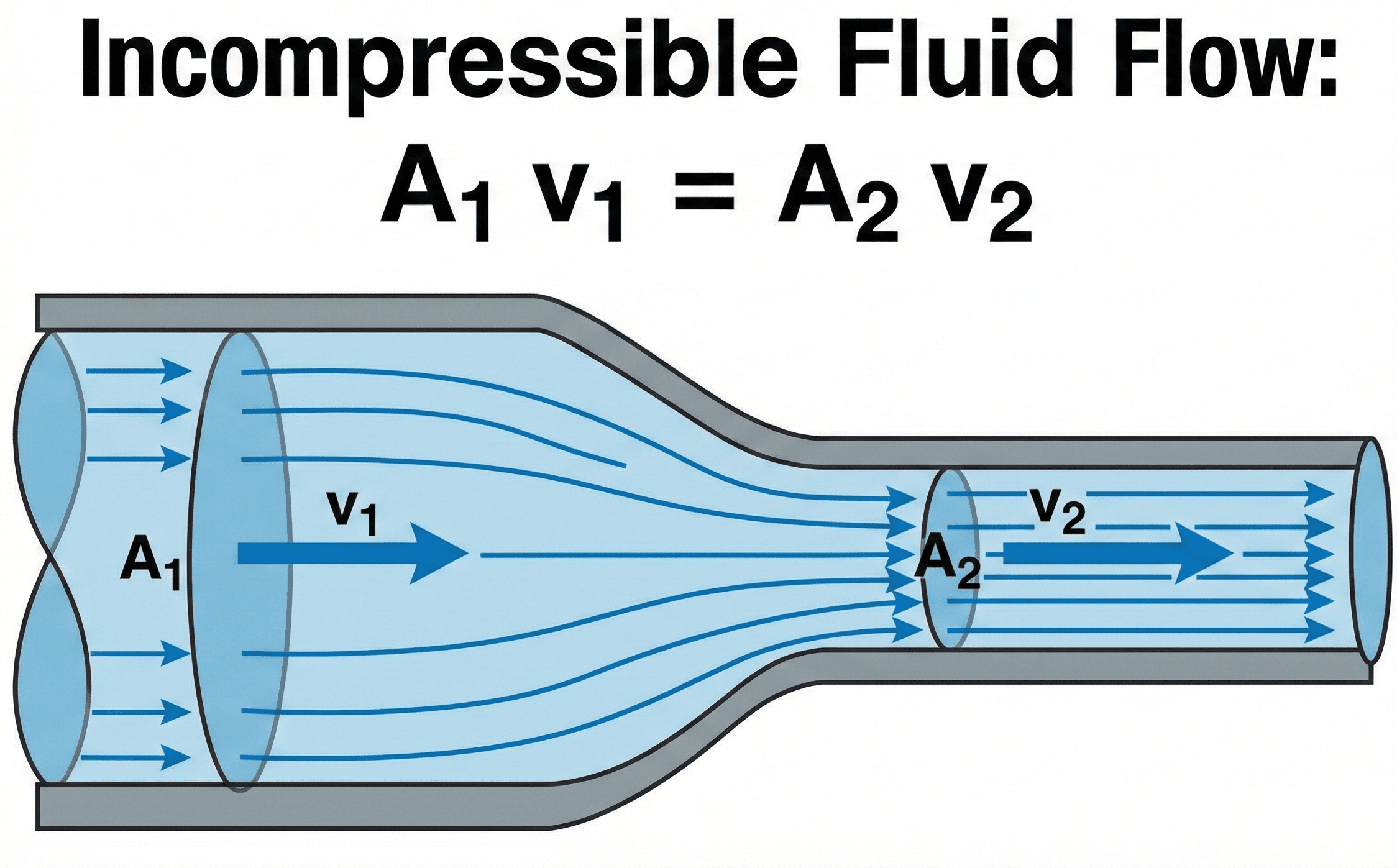
The first thing to notice is that the streamtube gets smaller where the pipe necks down. For incompressible flow, the same volumetric flow must pass every section, so the smaller section needs a higher average velocity. That simple visual idea is why continuity is one of the first equations engineers reach for in fluid mechanics.
What is the continuity equation?
The continuity equation is the mathematical statement of mass conservation. In plain terms, mass cannot disappear or be created inside an ordinary flow passage, so whatever mass enters a control volume must either leave it or temporarily accumulate inside it.
In engineering work, continuity is used for quick flow checks, nozzle and diffuser problems, pipe sizing, ventilation calculations, pump-system analysis, and as a starting point before applying more detailed relationships such as Bernoulli’s equation or the Navier–Stokes equation. It is also one of the core building blocks behind control-volume analysis in thermodynamics and fluid mechanics.
The engineer’s real problem is usually not “What is continuity?” It is more practical: If area changes, what happens to velocity? Or If density changes too, which form of the equation should I use? That is why a useful continuity-equation reference needs more than the formula alone.
The continuity equation formula
The most general engineering form is written in terms of mass flow rate. For steady one-dimensional flow between two sections, continuity is:
Expanding mass flow rate gives:
When the fluid is incompressible and density stays essentially constant, density cancels and the form most students and practicing engineers recognize appears:
Physically, this means the same flow must pass through each cross section. If the available area gets smaller, the average flow speed must rise. If the area gets larger, the average flow speed must drop. That is the same mass-conservation idea whether you are analyzing a water pipe, a nozzle, a duct, or a simplified streamtube.
Variables and units
Continuity only works cleanly when each symbol is interpreted correctly. In most engineering problems, \(A\) is the flow area normal to the average velocity, \(V\) is the average bulk velocity, and \(\rho\) is the fluid density.
- \(A\) Cross-sectional flow area. Common SI unit: m\(^2\). Common US customary unit: ft\(^2\).
- \(V\) Average flow velocity through the section. Common SI unit: m/s. Common US customary unit: ft/s.
- \(\rho\) Fluid density. Common SI unit: kg/m\(^3\). Common US customary unit: lbm/ft\(^3\) when using mass-based units.
- \(Q\) Volumetric flow rate, where \(Q = AV\). Common SI unit: m\(^3\)/s. Common US customary unit: ft\(^3\)/s or gpm after conversion.
- \(\dot{m}\) Mass flow rate, where \(\dot{m} = \rho AV\). Common SI unit: kg/s. Common US customary unit: lbm/s.
Keep area and velocity in the same unit system before multiplying them. If you use diameter in inches and velocity in ft/s without converting, the resulting flow rate will be wrong.
If area shrinks by half in an incompressible-flow problem, average velocity should roughly double. That quick proportional check catches many arithmetic and unit errors immediately.
| Variable | Meaning | SI units | US customary units | Typical range | Notes |
|---|---|---|---|---|---|
| \(A\) | Flow area | m\(^2\) | ft\(^2\) | Highly problem-dependent | Use the actual open flow area, not the outside pipe size. |
| \(V\) | Average velocity | m/s | ft/s | Often 0.1 to 5 m/s in many water systems | Average velocity is not the same as local peak velocity in the profile. |
| \(\rho\) | Density | kg/m\(^3\) | lbm/ft\(^3\) | About 1000 for water near room temperature | Density changes matter in compressible gas flow and some thermal problems. |
| \(Q\) | Volumetric flow rate | m\(^3\)/s | ft\(^3\)/s, gpm | System-dependent | \(Q\) stays constant for steady incompressible flow through a closed conduit. |
How to rearrange the continuity equation
In real use, engineers usually rearrange continuity to solve for an unknown velocity, area, density, or flow rate. For incompressible steady flow, the most common solve-for forms are:
If density changes cannot be ignored, use the mass-flow form instead:
After rearranging, check whether the trend makes physical sense. A smaller downstream area should not produce a lower downstream velocity in a basic incompressible closed-pipe problem unless some other assumption has changed.
Where engineers use this equation
Continuity shows up almost everywhere fluids move. It is simple, but it is not trivial. Many larger analysis methods fail when the mass balance itself is set up incorrectly.
- Pipes, nozzles, and diffusers: relating flow area changes to velocity changes before using pressure or head equations.
- HVAC and ductwork: checking air velocity as duct sizes change through branches, transitions, and fittings.
- Pumps and system curves: pairing continuity with Bernoulli’s equation and head-loss relationships to understand how flow moves through a hydraulic system.
- Control-volume analysis: establishing inflow, outflow, and storage terms in open-system thermodynamics and fluid mechanics.
- Flow-regime interpretation: using velocity from continuity to evaluate Reynolds number and judge whether laminar or turbulent assumptions are appropriate.
In plant and facility work, the equation itself is rarely the limiting step. The usual issue is whether the assumed area, measured flow, or effective density actually reflects site conditions such as fouling, partial blockage, leakage, or nonuniform flow distribution.
Worked example
Example problem
Water flows steadily through a pipe contraction. At section 1, the pipe diameter is 0.20 m and the average velocity is 1.8 m/s. At section 2, the diameter narrows to 0.10 m. Assuming incompressible flow, find the average velocity at section 2.
First compute the area ratio. Because both sections are circular, area is proportional to diameter squared:
Now use the incompressible continuity equation \(A_1V_1=A_2V_2\):
The downstream velocity is higher because the same volumetric flow must pass through a section with one-fourth the area. That is exactly the behavior shown in the diagram at the top of the page.
A result of 7.2 m/s is plausible because the pipe diameter was cut in half, which reduced area by a factor of four. If your answer had been 3.6 m/s, you likely treated area as proportional to diameter instead of diameter squared.
Assumptions behind the equation
The continuity equation always comes from mass conservation, but the simplified form you use depends on the physical assumptions built into the problem.
- 1 For \(A_1V_1=A_2V_2\), density must remain essentially constant between sections.
- 2 The chosen areas must represent the actual flowing cross section, not a nominal geometric size with obstructions ignored.
- 3 Velocity is usually treated as a section-average value, which is an approximation of a nonuniform real velocity profile.
- 4 For the steady one-dimensional form, storage inside the control volume is neglected or assumed zero over the time interval of interest.
Neglected factors
Continuity by itself does not account for pressure losses, viscosity, shear stresses, pump work, elevation head changes, or turbulence effects. It only enforces mass balance. Those neglected effects matter when you need pressure, head, or force predictions rather than just kinematic flow relations.
- Compressibility: matters in higher-speed gas flows, strong pressure changes, and thermal systems where density is not constant.
- Nonuniform profiles: matter when entrance effects, separation, swirl, or recirculation make average-velocity assumptions weak.
- Leakage or side branches: matter whenever flow is added, removed, or distributed along the path rather than staying in a single closed streamtube.
When the simple continuity form breaks down
The compact form \(A_1V_1=A_2V_2\) is powerful, but it is not universal. It begins to fail when the underlying assumptions stop matching the physics.
Do not use \(A_1V_1=A_2V_2\) blindly for compressible gas flow, strong heating or cooling, multi-branch systems, or cases where mass is being stored, injected, or removed inside the control volume.
In those situations, step back to the mass-flow form \(\rho AV\) or to the full control-volume continuity statement. If density varies significantly, the “same \(Q\) everywhere” idea no longer holds even though mass is still conserved.
Common mistakes and engineering checks
- Using diameter directly instead of converting to area or using the diameter-squared ratio.
- Mixing SI and US customary units in the same substitution step.
- Applying the incompressible form when density actually changes enough to matter.
- Using pipe inside diameter incorrectly because nominal size was confused with actual flow diameter.
- Forgetting that continuity alone does not give pressure change, head loss, or pump requirements.
Ask two quick questions before trusting the result: Did the area change in the direction expected, and did the calculated velocity move in the opposite proportional direction for incompressible flow?
| Check item | What to verify | Why it matters |
|---|---|---|
| Units | Area, velocity, and density all come from one consistent system. | Unit inconsistency is one of the fastest ways to destroy an otherwise correct setup. |
| Magnitude | The velocity change matches the area ratio trend. | If the direction of change is wrong, the algebra or geometry is probably wrong too. |
| Model choice | The selected form matches the actual density behavior and control-volume conditions. | Using the wrong form gives a clean-looking answer that may still be physically invalid. |
Continuity equation vs. related equations
Continuity is often taught beside other fluid equations, but each one answers a different engineering question. Knowing the distinction helps you choose the right tool quickly.
| Equation / method | Best used for | Key assumption | Main limitation |
|---|---|---|---|
| Continuity equation | Mass balance, flow-rate relationships, velocity-area changes | Mass is conserved in the chosen control volume | Does not by itself predict pressure or energy losses |
| Bernoulli’s equation | Relating pressure, velocity, and elevation along a streamline | Commonly assumes steady, incompressible, low-loss flow unless extended | Can be misused if losses, pumps, or viscous effects are ignored |
| Reynolds number | Determining flow regime and selecting correlations | Uses a representative length scale and velocity | It classifies flow behavior but is not a conservation equation |
| Navier–Stokes equation | First-principles momentum modeling of real fluid motion | Requires a stronger field description and more boundary information | Too complex for many hand calculations without simplification |
Frequently asked questions
The continuity equation is the mathematical statement of conservation of mass. It says the mass flow rate entering a control volume must equal the mass flow rate leaving it, unless mass is accumulating inside.
You can use \(A_1V_1 = A_2V_2\) when the fluid density is effectively constant, which is the standard incompressible-flow assumption for liquids and many low-speed gas problems.
Use any consistent unit system. Area and velocity must match so the volumetric flow rate has units of volume per time, such as m\(^3\)/s or ft\(^3\)/s. If density is included, the result becomes mass flow rate such as kg/s or lbm/s.
The continuity equation enforces conservation of mass, while Bernoulli’s equation relates pressure, velocity, and elevation through conservation of mechanical energy along a streamline under appropriate assumptions.
Summary and next steps
The continuity equation is one of the most important relationships in fluid mechanics because it forces every analysis to respect mass conservation. In practice, it connects area, velocity, density, and flow rate and often provides the first reliable equation in a larger problem.
The key judgment point is choosing the right form. Use \(A_1V_1=A_2V_2\) only when density is essentially constant. Step back to \(\rho AV\) or the full control-volume form when compressibility, storage, branching, or mass addition matters.
Where to go next
Continue the most useful learning path from basic mass conservation into broader fluid-system analysis.
-
Prerequisite: Reynolds Number
Use velocity from continuity to classify flow regime and choose reasonable next-step correlations.
-
Current topic: Continuity Equation
Return here when you need a quick mass-balance reference, rearrangement, or worked example.
-
Advanced: Bernoulli’s Equation
Move next into pressure, velocity, and elevation relationships once the mass balance is established.