
Key Takeaways
- Speed change: for the same centrifugal pump geometry, flow scales with speed, head with speed squared, and power with speed cubed.
- Practical use: engineers use the laws for VFD changes, pump-curve shifts, preliminary motor checks, and first-pass operating-point estimates.
- Watch for: the actual operating point still depends on the system curve, efficiency, BEP location, NPSH margin, and driver capacity.
- Impeller trims: diameter-based scaling is a useful estimate but usually less exact than speed scaling on the same pump.
Table of Contents
How pump affinity laws scale centrifugal-pump performance
Pump affinity laws compare a known operating condition with an estimated condition after changing rotational speed or, with more caution, impeller diameter.
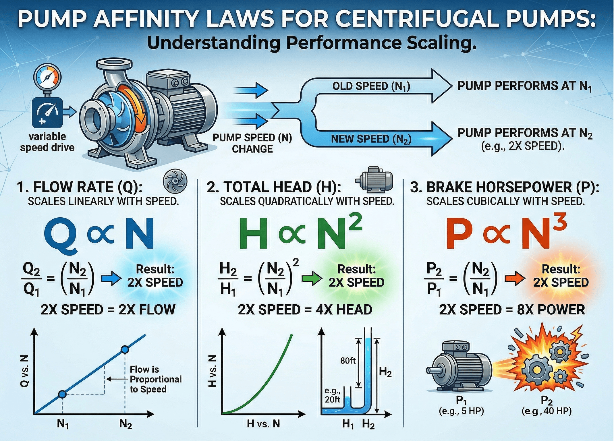
The cubic power relationship is the most important operational warning: a modest speed increase can create a much larger change in required shaft power.
What are pump affinity laws?
Pump affinity laws are similarity relationships used to estimate how centrifugal-pump performance changes when rotational speed or characteristic impeller size changes. They are most dependable when comparing the same pump at two nearby speeds with similar fluid properties.
The laws are commonly used with variable frequency drives, preliminary pump-curve shifts, operating-point estimates, and motor-load checks. They are not a replacement for the manufacturer’s pump curve or a complete hydraulic-system analysis.
Pump affinity laws formulas
For the same pump geometry operating at two different rotational speeds:
A 10% speed increase gives about 10% more idealized flow, 21% more head, and 33.1% more power demand.
Variables and units
- \(Q\)Volumetric flow rate, such as gpm, L/s, or m³/h.
- \(H\)Developed pump head, typically ft or m of fluid.
- \(P\)Pump shaft or brake power, commonly hp or kW.
- \(N\)Rotational speed, typically rpm.
- \(D\)Impeller diameter when using diameter-based scaling.
| Symbol | Meaning | Typical units | Engineering note |
|---|---|---|---|
| \(Q\) | Flow rate | gpm, L/s, m³/h | Use the same unit at conditions 1 and 2. |
| \(H\) | Head | ft, m | Head scales with the square of the speed ratio. |
| \(P\) | Shaft power | hp, kW | Power scales with the cube of the speed ratio. |
| \(N\) | Speed | rpm | Only the ratio matters in the ideal laws. |
| \(D\) | Impeller diameter | in, mm | Diameter scaling is more approximate for trims. |
Speed changes with a VFD
Speed scaling is the cleanest and most common pump-affinity application. If geometry and fluid properties are unchanged, define the speed ratio:
Then:
Increasing speed can overload the motor quickly because power rises with the cube of speed. Always compare predicted shaft power with motor capability and the actual pump curve.
Impeller-diameter affinity estimates
Diameter-based forms are often used as a first estimate for impeller trims:
Treat these as screening estimates. Trimming changes the hydraulic geometry, so actual efficiency and curve shape may depart from ideal scaling.
For a trimmed impeller, use the manufacturer’s trimmed performance curve whenever available.
Pump curve vs system curve
Affinity laws shift the pump’s expected performance, but the actual operating point is determined by the intersection of the pump curve and the system curve.
In a friction-dominated system, increasing flow raises system head rapidly. That means the real operating point after a speed change is not simply “old flow times the speed ratio” unless the shifted pump curve and system curve support that point.
Use the affinity laws to shift the pump curve, then find the new intersection with the system curve for a more realistic operating estimate.
BEP, efficiency, and acceptable operating range
Best efficiency point (BEP) is the region where the pump typically operates most efficiently and often most smoothly. Changing speed or system resistance can move the operating point away from BEP even when the affinity-law math is correct.
- Efficiency: do not assume pump efficiency remains exactly constant after a large operating change.
- Vibration and recirculation: operating too far left or right on the curve can increase hydraulic instability.
- Motor loading: verify shaft power at the new point, not only the ideal cubic estimate.
NPSH and cavitation checks after a speed change
Increasing pump speed can also increase suction-side risk. Net positive suction head required can rise as operating conditions change, while the system’s NPSH available may not improve.
Never approve a higher speed from affinity laws alone. Compare NPSH available with the manufacturer’s NPSH required data at the new operating condition.
Useful pump affinity law rearrangements
The flow relationship is often used backward to estimate a target speed:
If target head is known:
If target power is the limiting quantity:
Worked examples
Example 1: speed increase
A pump delivers \(500\ \text{gpm}\) at \(80\ \text{ft}\) of head and requires \(20\ \text{hp}\) at \(1750\ \text{rpm}\). Estimate performance at \(2100\ \text{rpm}\).
The ideal estimate is \(600\ \text{gpm}\), \(115.2\ \text{ft}\), and about \(34.6\ \text{hp}\). The power increase is about 73%, so driver capacity must be checked before increasing speed.
Example 2: impeller trim estimate
A pump with a \(10\ \text{in}\) impeller delivers \(900\ \text{gpm}\) at \(120\ \text{ft}\) and uses \(40\ \text{hp}\). Estimate the ideal result for a \(9\ \text{in}\) trim.
Use this only as a first-pass estimate. Final values should come from the manufacturer’s trimmed impeller curve.
Example 3: find speed for a target flow
A pump delivers \(400\ \text{gpm}\) at \(1450\ \text{rpm}\). Estimate the speed needed for \(460\ \text{gpm}\).
The corresponding ideal head multiplier is \(1.3225\), while the ideal power multiplier is \(1.5209\). A 15% flow increase therefore implies about 32% more head and 52% more power under ideal scaling.
Assumptions and limitations
- 1The pump is centrifugal and the compared operating conditions are reasonably similar.
- 2Fluid properties are similar enough that large viscosity or density changes do not invalidate the comparison.
- 3The pump remains within a practical region of its performance curve.
- 4Efficiency changes are not assumed away for final design.
- 5System curve, BEP, NPSH, and motor limits are checked separately.
Be cautious with large speed changes, cavitation-limited operation, viscous fluids, unusual impeller trims, non-similar pumps, or operating points near the ends of the pump curve.
Common mistakes and engineering checks
- Using the ideal affinity result as the actual system operating point without checking the system curve.
- Ignoring the cubic rise in power and motor loading.
- Assuming efficiency remains unchanged after a large operating shift.
- Using diameter-based scaling as if it were exact manufacturer data.
- Ignoring BEP and acceptable operating range.
- Failing to check NPSH margin after a speed increase.
| Check item | What to verify | Why it matters |
|---|---|---|
| Speed ratio | Use the correct baseline and target RPM | Every other ideal scaling result depends on it |
| Power | Check motor and driver capacity | Power changes with the cube of speed |
| System curve | Find the new pump/system intersection | Determines the actual operating point |
| BEP | Check where the new point lies on the pump curve | Efficiency and reliability can change materially |
| NPSH | Compare available vs required | Prevents cavitation risk from being overlooked |
Frequently asked questions
For the same centrifugal pump at different speeds, flow varies approximately with speed, head with speed squared, and power with speed cubed.
Yes. Speed-based affinity laws are commonly used to estimate how a centrifugal pump will shift when a VFD changes rotational speed, but the new operating point should still be checked against the system curve and manufacturer data.
They are useful as a first estimate, but impeller-diameter scaling is generally less exact than speed scaling. Use the manufacturer’s trimmed performance curve for final values.
Under ideal affinity scaling, shaft power varies with the cube of rotational speed. That is why even a modest speed increase can create a much larger increase in motor load.
No. The actual operating point is where the pump curve intersects the system curve, so affinity laws should be combined with pump-curve and system-curve analysis.
Summary and next steps
Pump affinity laws are powerful first-pass scaling relationships for centrifugal pumps. For speed changes, flow scales approximately with \(N\), head with \(N^2\), and power with \(N^3\).
The most important engineering judgment is knowing that the equations only shift expected pump performance. Final operating behavior still depends on the system curve, pump efficiency, BEP, NPSH margin, manufacturer data, and motor capacity.
Where to go next
-
Bernoulli Equation Calculator
Connect pump head to pressure, elevation, and velocity changes.
-
Hazen-Williams Calculator
Estimate pipe friction losses that shape the system curve.
-
Continuity Equation
Relate flow rate, velocity, and pipe area in the surrounding system.