Mechanical Engineering · Pump Affinity Laws
Pump Affinity Laws Formula – How to Calculate Flow, Head, and Power Changes
Learn the pump affinity laws formula engineers use to estimate how flow, head, and power change when centrifugal pump speed or impeller diameter changes, plus worked examples, limits, and when the equations stop being reliable.
Pump affinity laws formula: the direct answer and when to use it
Core formulas
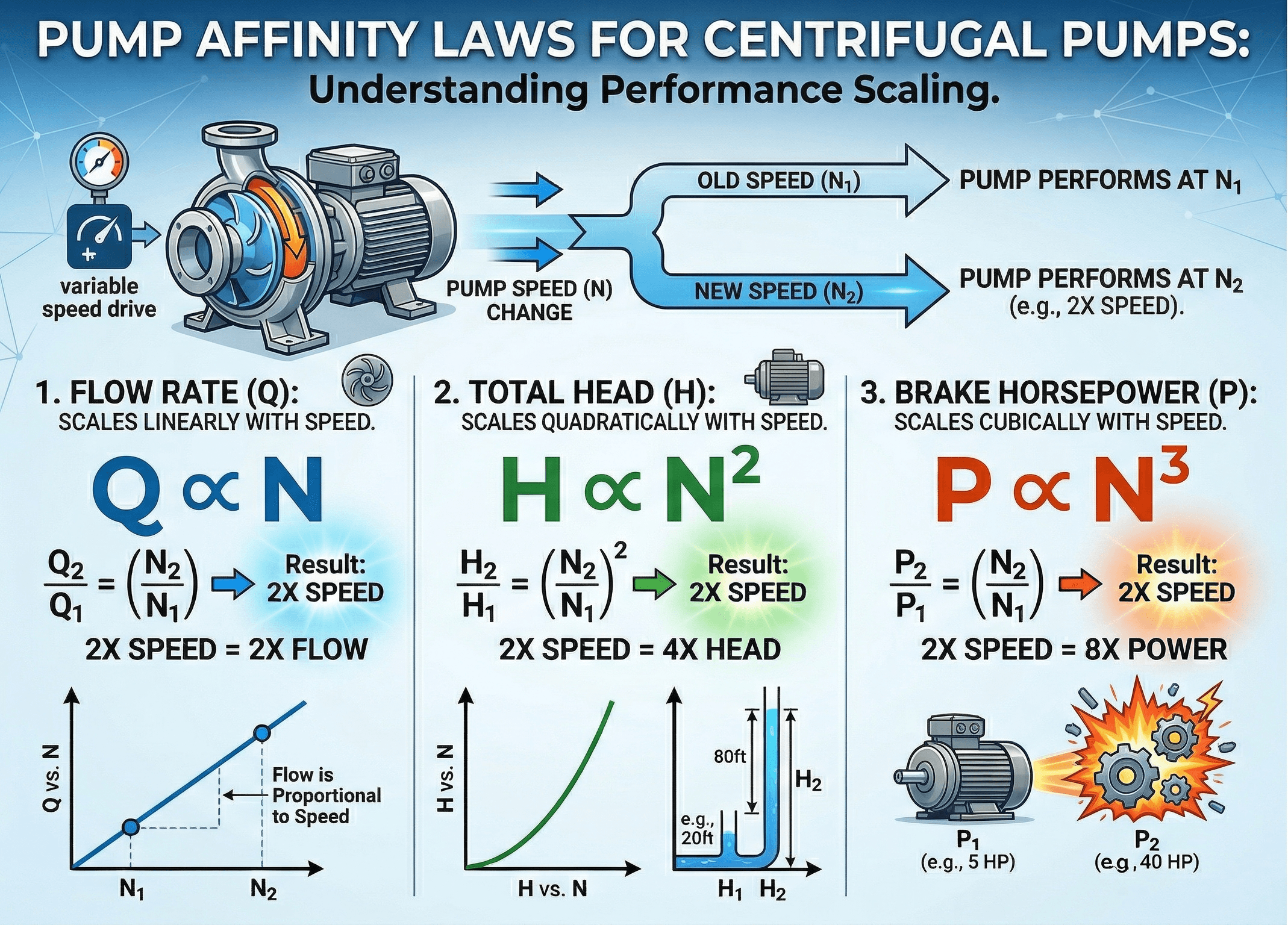
The pump affinity laws estimate how a centrifugal pump’s flow, head, and power change when speed changes and the pump geometry stays the same.
Most readers want this first: if pump speed increases by 10%, flow increases by about 10%, head increases by about 21%, and power increases by about 33%. The power change matters most in real systems because it rises much faster than flow.
The pump affinity laws are one of the most useful shortcut tools in pump engineering. They are commonly used for centrifugal pumps to estimate how operating conditions shift when speed changes. The laws are especially valuable in systems with variable frequency drives, where operators want to know how a new RPM will affect flow rate, developed head, and brake horsepower before changing the setpoint.
These equations are powerful because they answer the practical question searchers usually have: “What happens if I run the same pump faster or slower?” But they are estimation laws, not a substitute for a pump curve. They work best when the pump geometry is unchanged, the fluid remains similar, and the operating point stays within a reasonable region of the pump’s performance map.
Editorial note: this page is written for practical engineering use. The formulas are correct for ideal affinity-law scaling, but real pump selection still requires checking the pump curve, system curve, efficiency shift, NPSH limits, and motor capacity before relying on the estimate.
Pump affinity laws variables, units, and notation
The affinity laws compare a known pump operating point to a second estimated operating point. The subscripts matter: condition 1 is your baseline, and condition 2 is your predicted new condition after changing speed or diameter.
Common notation
| Symbol | Meaning | Typical unit | What it represents |
|---|---|---|---|
| \(Q\) | flow rate | gpm, L/s, m³/h | The volumetric flow delivered by the pump at a given operating point. |
| \(H\) | head | ft, m | The developed pump head, often treated as total dynamic head across the pump. |
| \(P\) | power | hp, kW | The shaft power or brake power required to drive the pump. |
| \(N\) | rotational speed | rpm | The impeller rotational speed of the pump. |
| \(D\) | impeller diameter | in, mm | The impeller outside diameter when using diameter-based scaling estimates. |
| BEP | best efficiency point | — | The region where the pump operates most efficiently and often most reliably. |
Unit and usage notes
- Because the laws use ratios, any consistent flow unit works as long as both conditions use the same unit.
- Head should be compared in the same unit at both operating points.
- Power should stay in one unit system for the comparison, usually hp or kW.
- Speed is normally in RPM, but only the speed ratio matters for the formula.
- Diameter-based forms are useful for first estimates, but real trimmed impellers often depart from ideal scaling more than simple speed changes do.
Pump affinity law estimates become much more useful when paired with head-loss calculations and fluid energy balance. For related system analysis, see the Bernoulli Equation Calculator.
How pump affinity laws work in practice
The main reason the affinity laws matter is that centrifugal pumps do not respond linearly in every way when speed changes. Flow is roughly linear with speed, but head follows the square relationship and power follows the cube relationship. That means the “cost” of increasing speed is usually felt most strongly in power demand.
Method 1: Changing speed on the same centrifugal pump
This is the most common real-world use. An operator has a known duty point at one speed and wants a quick estimate at a new speed. This happens constantly with VFD-controlled pumps in HVAC systems, water plants, industrial process loops, and irrigation systems.
For example, if speed rises from 1200 rpm to 1500 rpm, the speed ratio is 1.25. Flow rises by 25%, head rises by 56.25%, and power rises by about 95.3%. That is why a modest RPM increase can become a very serious motor or thermal issue if it is not checked carefully.
Method 2: Using diameter-based affinity estimates for impeller trims
The same pattern is often applied to impeller diameter changes as a first estimate. This is useful when evaluating trimmed impellers, but it is less exact than a speed-change estimate on the same pump because trimming changes the hydraulic geometry more directly.
Use this as a screening tool, not a final procurement value. If an impeller is trimmed, the vendor’s trimmed performance curve is the better reference because efficiency, slip, and actual hydraulic behavior may differ from the idealized ratio-based estimate.
The most important practical idea is that the affinity laws shift the pump’s expected performance, but the actual operating point still depends on the system curve. The pump and system must still intersect somewhere physically achievable. That is why affinity-law math and pump-curve reading belong together, not as separate topics.
Worked examples for pump affinity laws
These examples are arranged around the search intents that matter most: how to calculate a new operating point, how to estimate an impeller trim, and how to work backward to a required speed.
Example 1: Predict flow, head, and power after a speed increase
Scenario: A centrifugal pump delivers 500 gpm at 80 ft of head and requires 20 hp at 1750 rpm. Estimate the new operating values at 2100 rpm.
Steps:
- Calculate the speed ratio \(N_2/N_1\).
- Multiply baseline flow by the speed ratio.
- Multiply baseline head by the square of the speed ratio.
- Multiply baseline power by the cube of the speed ratio.
Result: the estimated new point is 600 gpm, 115.2 ft of head, and 34.6 hp.
Interpretation: this is the classic affinity-law lesson. A 20% speed increase gave a 20% flow increase, but the estimated power increase was nearly 73%. That is exactly why motor margin must be reviewed before raising speed.
Example 2: Estimate the effect of an impeller trim
Scenario: A pump with a 10 in impeller delivers 900 gpm at 120 ft of head and uses 40 hp. Estimate the new values if the impeller is trimmed to 9 in using the ideal diameter-based affinity form.
Steps:
- Compute the diameter ratio \(D_2/D_1\).
- Estimate flow from the first power of the ratio.
- Estimate head from the square of the ratio.
- Estimate power from the cube of the ratio.
Result: the ideal estimate gives 810 gpm, 97.2 ft of head, and 29.2 hp.
Interpretation: this is a useful first-pass trimmed impeller estimate, but it is not as dependable as a speed-change estimate. The next design step should be checking the manufacturer’s trimmed impeller curve.
Example 3: Find the speed needed for a target flow
Scenario: A pump delivers 400 gpm at 1450 rpm. You want about 460 gpm. Estimate the required speed and the resulting head and power multipliers.
Steps:
- Use the flow law to solve backward for the new speed.
- Use the same speed ratio to estimate head and power multipliers.
- Check whether the predicted power increase is acceptable for the driver.
Result: the required speed is about 1668 rpm. Head is estimated to rise by about 32.3%, and power by about 52.1%.
Interpretation: this is a good example of why seemingly small flow increases still require careful system and motor checks. The power penalty rises much faster than the flow target.
Common mistakes, assumptions, and engineering checks
The pump affinity laws are simple enough to memorize, but ranking-quality engineering content needs to show where they fail, where they help most, and what a careful reader should check next.
The affinity laws estimate how the pump performance shifts, but the actual operating point is still determined by the intersection of the pump curve and system curve. Without that check, the predicted point may not be physically where the pump will run.
- Use the laws to shift the expected pump behavior, not to replace system analysis.
- Review total dynamic head and friction losses at the new flow.
- Remember that a different flow means a different system-loss condition.
The cubic power relationship is the main reason these laws matter operationally. But motor load is not the only concern. A changed operating point can also move the pump away from best efficiency point, reduce efficiency, and increase vibration or heat.
- Compare predicted power against motor nameplate capacity and service factor.
- Check whether the new point moves too far from BEP.
- Do not assume pump efficiency stays constant after a major operating shift.
The affinity laws are strongest for the same centrifugal pump at a different speed. They are weaker for trimmed impellers, large operating shifts, non-similar geometry, unusual fluids, cavitation-limited cases, or conditions near the edge of the pump curve.
- Check NPSH available versus required after speed changes.
- Use manufacturer curves for trimmed impellers and final selections.
- Be cautious with large changes that move far from the original operating region.
Pump Affinity Laws FAQ
What are the three pump affinity laws?
For a similar centrifugal pump, flow varies directly with speed, head varies with the square of speed, and power varies with the cube of speed. They are commonly written as \(Q \propto N\), \(H \propto N^2\), and \(P \propto N^3\).
What is the pump affinity laws formula?
The most common speed-based forms are \(Q_2/Q_1=N_2/N_1\), \(H_2/H_1=(N_2/N_1)^2\), and \(P_2/P_1=(N_2/N_1)^3\). These compare a known pump operating point to a new estimated operating point.
Do pump affinity laws work for impeller trimming?
They work as a first estimate, but diameter-based predictions are usually less exact than speed-change predictions on the same pump. Trimmed impeller performance should be checked against the manufacturer’s curve for better accuracy.
Can I use affinity laws alone to size a pump?
No. They are best used for fast estimates. Final pump selection should also include the pump curve, system curve, efficiency, BEP location, NPSH limits, and driver capacity.
References and further reading
- Pump and Fan Affinity Laws | Engineering ToolBox – quick reference for the standard speed and diameter scaling relationships.
- Affinity Laws | KSB Centrifugal Pump Lexicon – manufacturer-oriented explanation of how centrifugal pump performance scales.
- Pump Affinity Laws Explained | Crest Pumps – practical overview with operating guidance and examples.
- Bernoulli Equation Calculator | Turn2Engineering – useful for relating pump head to pressure, elevation, and velocity changes in a system.
- Hazen-Williams Calculator | Turn2Engineering – useful for understanding how pipe friction affects the system side of pump operation.