Key Takeaways
- Traffic flow theory explains congestion: It connects speed, flow, and density so engineers can understand free-flow, capacity, breakdown, queues, and stop-and-go waves.
- The core equation is simple: The relationship \(q = kv\) links flow \(q\), density \(k\), and speed \(v\), but interpreting it correctly requires careful units and context.
- The fundamental diagram is the main visual: It shows why flow rises at low density, peaks near capacity, and drops once congestion forms.
- Shockwaves explain queue movement: Congestion waves often move upstream, which is why a slowdown can reach drivers before they see the bottleneck.
Table of Contents
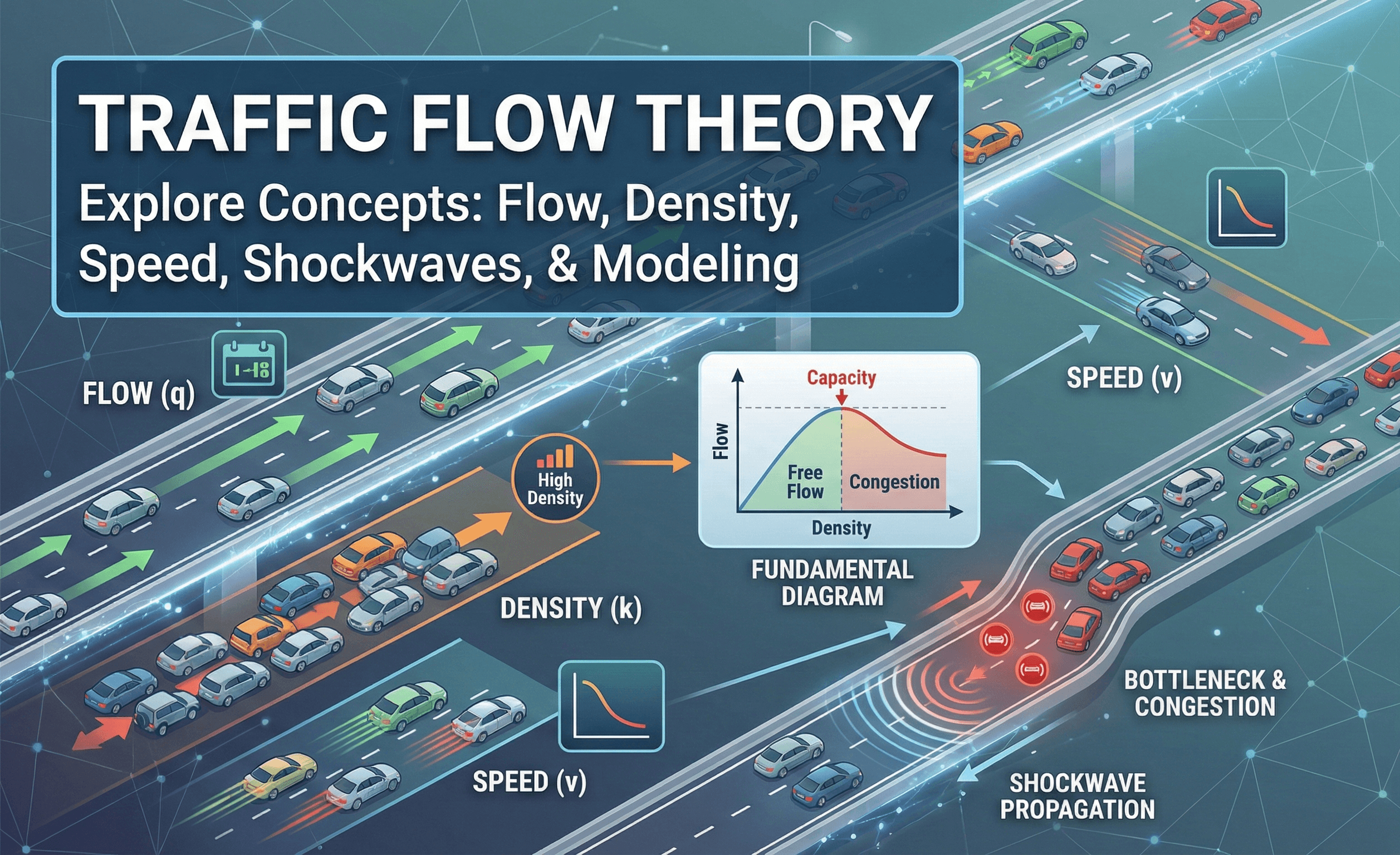
Featured diagram
Introduction
If you searched for traffic flow theory, you are probably trying to understand the “why” behind traffic behavior: why traffic slows down before a bottleneck, why stop-and-go waves appear with no crash, why adding vehicles can reduce throughput, and how engineers estimate roadway capacity.
Traffic flow theory answers those questions by treating traffic as a measurable stream. Instead of looking at only one driver or one car, it studies how many vehicles pass a point, how fast they move, how tightly they are packed, and how those conditions change as demand rises.
This guide is written for engineering students, transportation engineers, and technically curious readers who want a practical explanation. You will learn the core variables, the fundamental diagram, capacity and breakdown, shockwaves, queue growth, macroscopic vs. microscopic modeling, and how these ideas show up in real traffic engineering work.
What is Traffic Flow Theory?
Direct answer: Traffic flow theory is the study of how vehicles move as a traffic stream using relationships between flow, speed, and density. Engineers use it to estimate roadway capacity, understand congestion, identify bottlenecks, evaluate queues, and explain why traffic breakdown and stop-and-go waves can occur even without a crash.
The simplest version of the theory says that traffic flow depends on how many vehicles occupy a roadway and how fast they are moving. The harder part is interpreting what happens near capacity, where small disturbances can cause speeds to collapse and queues to grow upstream.
By the end of this page, you should be able to read a fundamental diagram, calculate density from flow and speed, interpret shockwave direction, and recognize why near-capacity traffic is fragile.
Core variables in Traffic Flow Theory
Nearly every practical traffic flow concept starts with three variables: flow, speed, and density. These variables describe how much traffic is moving, how fast it is moving, and how tightly vehicles are spaced on the roadway.
- \(q\) Flow rate: vehicles per hour (veh/h) or vehicles per hour per lane (veh/h/ln)
- \(v\) Mean speed: miles per hour (mph), kilometers per hour (km/h), feet per second (ft/s), or meters per second (m/s)
- \(k\) Density: vehicles per mile per lane (veh/mi/ln) or vehicles per kilometer per lane (veh/km/ln)
This equation is simple, but it is the foundation of traffic flow theory. If density increases while speed remains high, flow increases. But once density becomes too high, vehicles interfere with each other, speed drops, and flow can eventually decrease.
Always state the units. If \(q\) is in vehicles per hour per lane and \(v\) is in miles per hour, then \(k = q/v\) gives vehicles per mile per lane.
Time-mean speed vs. space-mean speed
In traffic data, “average speed” can mean different things. This matters because traffic flow calculations often require a speed that represents movement over a segment, not just spot speeds at one point.
| Speed type | What it means | Typical source | Why it matters |
|---|---|---|---|
| Time-mean speed | Average of spot speeds measured at a point | Radar, loop detector, point sensor | Useful for spot-speed studies, but can overrepresent faster vehicles |
| Space-mean speed | Average speed over a roadway segment based on travel time | Probe data, floating car runs, travel time sensors | More useful for flow-density relationships and segment operations |
| Free-flow speed | Speed under low-density, unconstrained conditions | Field studies, HCM procedures, agency assumptions | Used to define baseline operating conditions and capacity relationships |
| Operating speed | Speed drivers actually choose under prevailing conditions | Speed studies, probe data, observations | Important for safety, design consistency, and congestion diagnosis |
Do not mix point-based speed data with segment-based density or travel-time data without understanding the definitions. The math may still “work,” but the interpretation can be wrong.
Worked example: calculating density from flow and speed
Example
Suppose a freeway lane carries \(q = 1{,}800\) veh/h/ln at an average speed of \(v = 45\) mph. Estimate the traffic density.
A density of \(40\) veh/mi/ln means vehicles are interacting significantly. This may not be full stop-and-go congestion, but it is no longer an empty-road free-flow condition. If this state occurs near a merge, lane drop, steep grade, or weaving area, the facility may be sensitive to breakdown.
The same density can behave differently depending on lane count, heavy vehicles, grades, weather, ramp spacing, and downstream bottlenecks. Traffic states should always be interpreted with roadway context.
The fundamental diagram of traffic flow
The fundamental diagram is the main visual model in traffic flow theory. It shows how traffic behavior changes as density increases. The most common views are flow vs. density, speed vs. density, and speed vs. flow.
The story is simple: at low density, vehicles travel freely and flow increases as more vehicles enter the road. Near capacity, the roadway carries its maximum sustainable flow. Beyond that point, additional vehicles create interference, speeds drop, queues form, and flow can decrease even as density continues to rise.
| Traffic regime | What drivers experience | What the diagram shows | Engineering meaning |
|---|---|---|---|
| Free-flow | High speeds, large gaps, easy lane changes | Low density, speed near free-flow speed | Demand is below the operational limit |
| Near capacity | High flow, smaller gaps, more sensitivity | Flow approaches maximum value | Small disturbances can trigger breakdown |
| Congested flow | Low speeds, queues, stop-and-go movement | High density, lower speeds, reduced flow | The facility is unstable or oversaturated |
| Jam condition | Traffic is nearly stopped | Very high density, near-zero speed | Storage is full and throughput is severely reduced |
Add a 16:9 infographic here showing flow-density, speed-density, and speed-flow curves with labels for free-flow, capacity, critical density, congested flow, and jam density. This is the highest-value visual for the page.
Simple speed-density model: Greenshields form
Many introductory traffic flow courses use a linear speed-density relationship to build intuition. Real traffic is not perfectly linear, but the model clearly shows the basic idea: speed decreases as density increases.
- \(v\) Traffic stream speed
- \(v_f\) Free-flow speed
- \(k\) Traffic density
- \(k_j\) Jam density, where traffic is essentially stopped
Combining this relationship with \(q = kv\) gives a parabolic flow-density curve:
This curve rises as density increases from very low values, reaches a maximum at capacity, and then drops as traffic becomes congested. That visual pattern is the core of the fundamental diagram.
Capacity, breakdown, and capacity drop
Capacity is the maximum sustainable rate at which traffic can pass a point under prevailing conditions. But in real traffic, capacity is not always a single fixed number. It depends on roadway geometry, driver behavior, heavy vehicles, grades, weather, incidents, lane changes, and downstream constraints.
What breakdown means
Breakdown is the transition from stable near-capacity flow to congested flow. When traffic is near capacity, small disturbances can grow instead of fading. A brief brake tap, merging conflict, or lane change can trigger a speed drop that spreads upstream.
Capacity drop
After breakdown, the discharge flow from a bottleneck is often lower than the flow that existed before breakdown. This is called capacity drop. It explains why congestion can be hard to clear once it starts.
Preventing breakdown is often easier than recovering from it. Ramp metering, speed harmonization, incident management, and lane-use control often aim to keep traffic stable before queues form.
Shockwaves: how traffic congestion moves upstream
A traffic shockwave is the moving boundary between two traffic states. For example, the back of a queue is a boundary between upstream moving traffic and downstream congested traffic. This boundary often moves upstream, which means drivers encounter the queue before they reach the actual bottleneck.
- \(w\) Shockwave speed
- \(q_1, q_2\) Traffic flow rates in states 1 and 2
- \(k_1, k_2\) Traffic densities in states 1 and 2
A negative \(w\) usually means the wave moves upstream. A positive \(w\) means it moves downstream. For queue analysis, the upstream movement of the back of a queue is often the key concern.
Worked example: estimating shockwave speed
Example
Suppose upstream traffic is flowing freely at \(q_1 = 1{,}800\) veh/h/ln and \(k_1 = 30\) veh/mi/ln. Downstream queued traffic has \(q_2 = 600\) veh/h/ln and \(k_2 = 120\) veh/mi/ln. Estimate the speed of the boundary between these two states.
The negative value means the wave moves upstream. In this example, the back of the queue is moving upstream at about \(13.3\) mph. That means the queue can reach upstream ramps, intersections, or lane drops even though the original bottleneck is downstream.
Shockwave speed is useful because it converts abstract traffic states into a practical question: how long until the queue reaches the next ramp, intersection, or decision point?
Headway, spacing, and occupancy
Traffic engineers often use headway, spacing, and occupancy to understand how tightly vehicles are moving. These concepts are especially useful when working with detectors and field data.
| Concept | Meaning | Typical units | Why it matters |
|---|---|---|---|
| Time headway | Time between two successive vehicles passing a point | seconds/vehicle | Useful for estimating flow and following behavior |
| Space headway | Distance between two successive vehicles at a moment in time | feet/vehicle or meters/vehicle | Related to density and spacing in the traffic stream |
| Spacing | Physical distance between vehicles | feet or meters | Helps describe how tightly vehicles are packed |
| Occupancy | Percent of time a detector is occupied by vehicles | percent | Often used as a proxy for density, but requires careful interpretation |
In this simplified relationship, \(h\) is average time headway in seconds per vehicle and \(q\) is flow in vehicles per hour. For example, a 2-second average headway corresponds to about \(1{,}800\) vehicles per hour.
Occupancy is not the same as density. It depends on vehicle length, detector length, and speed. Treat occupancy-based density estimates carefully unless the detector has been calibrated.
Bottlenecks and queue growth
A bottleneck is a location where traffic demand exceeds the discharge capacity of a roadway element. Bottlenecks can be caused by geometry, control, incidents, work zones, weather, grades, merges, lane drops, or downstream congestion.
| Bottleneck type | Typical cause | Traffic flow theory concept | Possible operational response |
|---|---|---|---|
| Lane drop | Reduced number of lanes | Capacity reduction and queue formation | Advance signing, merge control, lane management |
| Ramp merge | Entering traffic increases density | Breakdown near capacity | Ramp metering, auxiliary lane, merge improvements |
| Steep grade | Heavy vehicles slow down | Moving bottleneck and speed disturbance | Truck climbing lane, speed management |
| Signalized intersection | Red time interrupts flow | Queue storage and discharge flow | Signal timing, coordination, turn-lane storage |
| Work zone | Lane closure or narrowed lanes | Reduced capacity and shockwaves | Off-peak closures, queue warning, detours |
| Incident | Blocked lane or driver distraction | Temporary capacity drop | Incident response, traveler information, clearance strategy |
In many real projects, the important question is not just “what is the capacity?” but “where will the queue go once demand exceeds capacity?”
Macroscopic vs. microscopic traffic flow models
Traffic flow theory can be applied at different levels of detail. The right approach depends on the question, the available data, and whether the goal is screening, design, operations, or research.
| Model type | How it treats traffic | Best for | Limitations |
|---|---|---|---|
| Macroscopic | Traffic as an aggregate stream | Flow, speed, density, capacity, queue propagation | Does not model individual driver behavior in detail |
| Microscopic | Individual vehicles and driver interactions | Lane changes, car-following, ramps, weaving, intersections | Requires calibration and many assumptions |
| Mesoscopic | Hybrid between aggregate flow and individual vehicle movement | Larger networks where full microsimulation is too heavy | Less detailed than microsimulation |
| Kinematic-wave | Traffic waves based on conservation and flow-density relationships | Shockwaves, queues, bottlenecks, spillback | Requires careful traffic-state assumptions |
If you need to understand “how much” flow a facility can handle, start macroscopic. If you need to understand lane-by-lane interactions, merges, or driver behavior, microscopic tools may be needed.
Where Traffic Flow Theory is used in real projects
Traffic flow theory is not just classroom math. It appears in freeway operations, signal timing, work zone planning, bottleneck diagnosis, traffic impact studies, incident response, and capacity analysis.
| Application | What the theory explains | Typical engineering decision |
|---|---|---|
| Freeway bottleneck | Breakdown, capacity drop, and queue growth | Ramp metering, auxiliary lanes, incident management |
| Signalized corridor | Platoons, queues, discharge flow, and spillback | Signal timing, coordination, turn-lane storage |
| Work zone | Reduced capacity and upstream shockwaves | Lane-closure timing, detours, queue warning systems |
| Ramp merge | Density increase and turbulence near merge areas | Ramp metering, merge design, auxiliary lane evaluation |
| Incident response | Temporary capacity loss and queue propagation | Clearance priority, traveler information, emergency routing |
| Traffic impact study | How added demand affects operations | Mitigation, access management, turn lanes, signal changes |
| Managed lanes | Demand control and stable flow maintenance | Pricing, access points, occupancy restrictions, ramp control |
For the broader applied discipline, see Traffic Engineering.
Common mistakes and quick engineering checks
Traffic flow theory becomes useful when it helps you avoid wrong conclusions from messy field data. The most common mistakes usually involve units, definitions, detector data, or applying the wrong traffic regime.
| Common mistake | Why it causes problems | Quick engineering check |
|---|---|---|
| Mixing total flow and per-lane flow | Density and capacity estimates become inconsistent | Always label flow as veh/h or veh/h/ln |
| Using mph with metric density | Units no longer cancel correctly | Convert units before calculating \(q = kv\) |
| Treating occupancy as density | Occupancy depends on speed and vehicle length | Use calibration or compare with probe data |
| Assuming capacity is constant | Weather, incidents, heavy vehicles, and merges change effective capacity | Use observed discharge rates when available |
| Ignoring regime changes | Free-flow assumptions do not work after breakdown | Identify whether traffic is free-flow, near-capacity, or congested |
| Ignoring downstream constraints | Upstream segment may look acceptable while downstream spillback controls operations | Trace queues and bottlenecks through the network |
When you compute a traffic state, write it as \((q, v, k)\) with units. If you cannot clearly state the units, the result is not ready for design or operations decisions.
How engineers apply Traffic Flow Theory
On real projects, engineers use traffic flow theory to interpret field data, diagnose bottlenecks, estimate queue growth, evaluate operational strategies, and explain why traffic behaves differently under free-flow and congested conditions.
- Define the facility and question: freeway segment, ramp merge, signalized corridor, lane drop, work zone, or bottleneck.
- Collect traffic data: flow, speed, occupancy, density estimates, queues, travel times, and incident observations.
- Identify the traffic regime: free-flow, near-capacity, congested, or queued.
- Compute traffic states: use \(q\), \(v\), and \(k\) to describe conditions clearly.
- Locate bottlenecks: identify where discharge capacity is lower than arrival demand.
- Estimate queue behavior: use shockwave logic to understand queue growth and spillback risk.
- Evaluate countermeasures: ramp metering, signal timing, lane management, work zone staging, or demand control.
- Validate against field conditions: compare calculations with observed queues, speeds, and travel times.
The best traffic flow analysis explains both the number and the physical behavior. If the math says a queue grows upstream, the field review should show where that queue would go and what it would block.
Relevant standards and design references
Traffic flow theory shows up in the methods and tools transportation engineers use to evaluate capacity, operations, performance, and traffic control. The exact reference depends on the facility type and agency.
- Highway Capacity Manual (HCM): Core reference for capacity and operational analysis of freeways, highways, intersections, ramps, streets, and multimodal facilities. Review the HCM 7th Edition overview.
- FHWA Traffic Analysis Tools: FHWA provides resources for traffic operations analysis tools, modeling guidance, and method selection. Explore FHWA Traffic Analysis Tools.
- Manual on Uniform Traffic Control Devices (MUTCD): The national standard for traffic control devices such as signs, signals, and pavement markings. Visit the official MUTCD site.
- FHWA traffic flow theory references: FHWA and transportation research references provide deeper background on traffic stream behavior, car-following, shockwaves, and modeling. Review FHWA Traffic Flow Theory resources.
- State and local agency manuals: Local methods may control accepted capacity assumptions, signal timing practices, detector data use, traffic impact study procedures, and operational thresholds.
Always verify the governing method before applying traffic flow theory to a real project. Agency procedures may define specific capacity values, default parameters, peak-hour factors, traffic data requirements, and acceptable tools.
Frequently asked questions
Traffic flow theory is used to relate speed, flow, and density so engineers can estimate capacity, understand congestion, diagnose bottlenecks, evaluate queue growth, and analyze freeway, arterial, ramp, and intersection operations.
The basic equation is \(q = kv\), where \(q\) is flow, \(k\) is density, and \(v\) is speed. It means traffic flow equals the number of vehicles occupying the roadway multiplied by how fast they are moving.
Traffic jams can form without a crash when traffic is near capacity and small disturbances such as braking, lane changes, merging, or slight capacity reductions amplify into stop-and-go waves that move upstream.
The fundamental diagram shows the relationship between flow, density, and speed. It explains free-flow conditions at low density, maximum flow near capacity, and reduced flow under congested high-density conditions.
A traffic shockwave is the moving boundary between two traffic states, such as free-flow traffic and queued traffic. Negative shockwave speed usually means the queue boundary is moving upstream.
Macroscopic models treat traffic as an aggregate stream using variables like flow, speed, and density. Microscopic models simulate individual vehicles and driver interactions such as car-following, lane-changing, and gap acceptance.
Summary and next steps
Traffic flow theory gives transportation engineers a practical way to understand how traffic behaves as demand changes. By connecting speed, flow, and density, it explains why roadways can operate smoothly at low density, become fragile near capacity, and break down into congestion once small disturbances begin to amplify.
The most important concept is that traffic is not just a count of vehicles. It is a dynamic stream. A facility can carry high flow under stable conditions, but once congestion starts, discharge can fall, queues can grow, and shockwaves can move upstream through the network.
To build mastery, practice computing traffic states, reading fundamental diagrams, interpreting shockwave direction, and connecting the math to field observations like queues, bottlenecks, speeds, and travel times.
Where to go next
Continue your learning path with these related transportation engineering resources.
-
Traffic Engineering
Learn how traffic flow concepts are applied to signal timing, traffic studies, capacity analysis, and safety improvements.
-
Highway Design
See how speed, capacity, geometry, sight distance, and design consistency shape roadway design decisions.
-
Transportation Planning
Understand how long-range demand forecasts and corridor planning connect to traffic operations.
-
Transportation Engineering hub
Browse more transportation resource pages and build your study path from fundamentals to applied design.